Parallel query support in PostgreSQL in the upcoming 9.6 release will be available for a number of query types: sequence scans, aggregates and joins. Because PostGIS tends to involve CPU-intensive calculations on geometries, support for parallel query has been at the top of our request list to the core team for a long time. Now that it is finally arriving the question is: does it really help?

TL;DR:

• With some adjustments to function COST both parallel sequence scan and parallel aggregation deliver very good parallel performance results.
• The cost adjustments for sequence scan and aggregate scan are not consistent in magnitude.
• Parallel join does not seem to work for PostGIS indexes yet, but perhaps there is some magic to learn from PostgreSQL core on that.

Setup

In order to run these tests yourself, you will need to check out and build:

• PostgreSQL 9.6 development code from the git master branch
• PostGIS 2.3 development code from this parallel enabled branch

For testing, I used the set of 69534polling divisions defined by Elections Canada.

shp2pgsql -s 3347 -I -D -W latin1 PD_A.shp pd | psql parallel

It’s worth noting that this data set is, in terms of number of rows very very small in database terms. This will become important as we explore the behaviour of the parallel processing, because the assumptions of the PostgreSQL developers about what constitutes a “parallelizable load” might not match our assumptions in the GIS world.

With the data loaded, we can do some tests on parallel query. Note that there are some new configuration options for parallel behaviour that will be useful during testing:

• max_parallel_degree sets the maximum degree of parallelism for an individual parallel operation. Default 0.
• parallel_tuple_cost sets the planner’s estimate of the cost of transferring a tuple from a parallel worker process to another process. The default is 0.1.
• parallel_setup_cost sets the planner’s estimate of the cost of launching parallel worker processes. The default is 1000.
• force_parallel_mode allows the use of parallel queries for testing purposes even in cases where no performance benefit is expected. Default ‘off’.

Parallel Sequence Scan

Before we can test parallelism, we need to turn it on! The default max_parallel_degree is zero, so we need a non-zero value. For my tests, I’m using a 2-core laptop, so:

SETmax_parallel_degree=2;

Now we are ready to run a query with a spatial filter. Using EXPLAIN ANALYZE suppressed the actual answer in favour of returning the query plan and the observed execution time:

EXPLAINANALYZESELECTCount(*)FROMpdWHEREST_Area(geom)>10000;

And the answer we get back is:

 Aggregate  
 (cost=14676.95..14676.97 rows=1 width=8) 
 (actual time=757.489..757.489 rows=1 loops=1)
   ->  Seq Scan on pd  
   (cost=0.00..14619.01 rows=23178 width=0) 
   (actual time=0.160..747.161 rows=62158 loops=1)
         Filter: (st_area(geom) > '10000'::double precision)
         Rows Removed by Filter: 7376
 Planning time: 0.137 ms
 Execution time: 757.553 ms

Two things we can learn here:

• There is no parallelism going on here, the query plan is just a single-threaded one.
• The single-threaded execution time is about 750ms.

Now we have a number of options to fix this problem:

• We can force parallelism using SET force_parallel_mode=on, or
• We can force parallelism by decreasing the parallel_setup_cost, or
• We can adjust the cost of ST_Area() to try and get the planner to do the right thing automatically.

It turns out that the current definition of ST_Area() has a default COST setting, so it is considered to be no more or less expensive than something like addition or substraction. Since calculating area involves multiple floating point operations per polygon segment, that’s a stupid cost.

In general, all PostGIS functions are going to have to be reviewed and costed to work better with parallelism.

If we redefine ST_Area() with a big juicy cost, things might get better.

CREATEORREPLACEFUNCTIONST_Area(geometry)RETURNSFLOAT8AS'$libdir/postgis-2.3','area'LANGUAGE'c'IMMUTABLESTRICTPARALLELSAFECOST100;

Now the query plan for our filter is much improved:

Finalize Aggregate  
(cost=20482.97..20482.98 rows=1 width=8) 
(actual time=345.855..345.856 rows=1 loops=1)
->  Gather  
   (cost=20482.65..20482.96 rows=3 width=8) 
   (actual time=345.674..345.846 rows=4 loops=1)
     Number of Workers: 3
     ->  Partial Aggregate  
         (cost=19482.65..19482.66 rows=1 width=8) 
         (actual time=336.663..336.664 rows=1 loops=4)
           ->  Parallel Seq Scan on pd  
               (cost=0.00..19463.96 rows=7477 width=0) 
               (actual time=0.154..331.815 rows=15540 loops=4)
                 Filter: (st_area(geom) > '10000'::double precision)
                 Rows Removed by Filter: 1844
Planning time: 0.145 ms
Execution time: 349.345 ms

Three important things to note:

• We have a parallel query plan!
• Some of the execution results output are wrong! They say that only 1844 rows were removed by the filter, but in fact 7376 were (as we can confirm by running the queries without the EXPLAIN ANALYZE). This is a known limitation, reporting on the results of only one parallel worker, which (should) maybe, hopefully be fixed before 9.6 comes out.
• The execution time has been halved, just as we would hope for a 2-core machine!

Now for the disappointing part, try this:

EXPLAINANALYZESELECTST_Area(geom)FROMpd;

Even though the work being carried out (run ST_Area() on 70K polygons) is exactly the same as in our first example, the planner does not parallelize it, because the work is not in the filter.

 Seq Scan on pd  
 (cost=0.00..31654.84 rows=69534 width=8) 
 (actual time=0.130..722.286 rows=69534 loops=1)
 Planning time: 0.078 ms
 Execution time: 727.344 ms

For geospatial folks, who tend to do a fair amount of expensive calculation in the SELECT parameters, this is a bit disappointing. However, we still get impressive parallelism on the filter!

Parallel Aggregation

The aggregate most PostGIS users would like to see parallelized is ST_Union() so it’s worth explaining why that’s actually a little hard.

PostgreSQL Aggregates

All aggregate functions in PostgreSQL consist of at least two functions:

• A “transfer function” that takes in a value and a transfer state, and adds the value to the state. For example, the Avg() aggregate has a transfer state consisting of the sum of all values seen so far, and the count of all values processed.
• A “final function” that takes in a transfer state and converts it to the final aggregate output value. For example, the Avg() aggregate final function divides the sum of all values by the count of all values and returns that number.

For parallel processing, PostgreSQL adds a third kind of function:

• A “combine” function, that takes in two transfer states and outputs a singe combined state. For the Avg() aggregate, this would add the sums from each state and counts from each state and return that as the new combined state.

So, in order to get parallel processing in an aggregate, we need to define “combine functions” for all the aggregates we want parallelized. That way the master process can take the completed transfer states of all parallel workers, combine them, and then hand that final state to the final function for output.

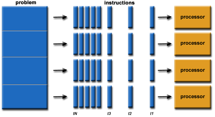
To sum up, in parallel aggregation:

• Each worker runs “transfer functions” on the records it is responsible for, generating a partial “transfer state”.
• The master takes all those partial “transfer states” and “combines” them into a “final state”.
• The master then runs the “final function” on the “final state” to get the completed aggregate.

Note where the work occurs: the workers only run the transfer functions, and the master runs both the combine and final functions.

PostGIS ST_Union Aggregate

One of the things we are proud of in PostGIS is the performance of our ST_Union() implementation, which gains performance from the use of a cascaded union algorithm.

Cascaded union involves the following steps:

• Collects all the geometries of interest into an array (aggregate transfer function), then
• Builds a tree on those geometries and unions them from the leaves of the tree upwards (aggregate final function).

Note that all the hard work happens in the final step. The transfer functions (which is what would be run on the workers) do very little work, just gathering geometries into an array.

Converting this process into a parallel one by adding a combine function that does the union would not make things any faster, because the combine step also happens on the master. What we need is an approach that does more work during the transfer function step.

PostGIS ST_MemUnion Aggregate

“Fortunately” we have such an aggregate, the old union implementation from before we added “cascaded union”. The “memory friendly” union saves memory by not building up the array of geometries in memory, at the cost of spending lots of CPU unioning each input geometry into the transfer state.

In that respect, it is the perfect example to use for testing parallel aggregate.

The non-parallel definition of ST_MemUnion() is this:

CREATEAGGREGATEST_MemUnion(basetype=geometry,sfunc=ST_Union,stype=geometry);

No special types or functions required: the transfer state is a geometry, and as each new value comes in the two-parameter version of the ST_Union() function is called to union it onto the state. There is no final function because the transfer state is the output value. Making the parallel version is as simple as adding a combine function that also uses ST_Union() to merge the partial states:

CREATEAGGREGATEST_MemUnion(basetype=geometry,sfunc=ST_Union,combinefunc=ST_Union,stype=geometry);

Now we can run an aggregation using ST_MemUnion() to see the results. We will union the polling districts of just one riding, so 169 polygons:

EXPLAINANALYZESELECTST_Area(ST_MemUnion(geom))FROMpdWHEREfed_num=47005;

Hm, no parallelism in the plan, and an execution time of 3.7 seconds:

 Aggregate  
 (cost=14494.92..14495.18 rows=1 width=8) 
 (actual time=3784.781..3784.782 rows=1 loops=1)
   ->  Seq Scan on pd  
   (cost=0.00..14445.17 rows=199 width=2311) 
   (actual time=0.078..49.605 rows=169 loops=1)
         Filter: (fed_num = 47005)
         Rows Removed by Filter: 69365
 Planning time: 0.207 ms
 Execution time: 3784.997 ms

We have to bump the cost of the two parameter version of ST_Union() up to 10000 before parallelism kicks in:

CREATEORREPLACEFUNCTIONST_Union(geom1geometry,geom2geometry)RETURNSgeometryAS'$libdir/postgis-2.3','geomunion'LANGUAGE'c'IMMUTABLESTRICTPARALLELSAFECOST10000;

Now we get a parallel execution! And the time drops down substantially, though not quite a 50% reduction.

 Finalize Aggregate  
 (cost=16536.53..16536.79 rows=1 width=8) 
 (actual time=2263.638..2263.639 rows=1 loops=1)
   ->  Gather  
   (cost=16461.22..16461.53 rows=3 width=32) 
   (actual time=754.309..757.204 rows=4 loops=1)
         Number of Workers: 3
         ->  Partial Aggregate  
         (cost=15461.22..15461.23 rows=1 width=32) 
         (actual time=676.738..676.739 rows=1 loops=4)
               ->  Parallel Seq Scan on pd  
               (cost=0.00..13856.38 rows=64 width=2311) 
               (actual time=3.009..27.321 rows=42 loops=4)
                     Filter: (fed_num = 47005)
                     Rows Removed by Filter: 17341
 Planning time: 0.219 ms
 Execution time: 2264.684 ms

The punchline though, is what happens when we run the query using a single-threaded ST_Union() with cascaded union:

EXPLAINANALYZESELECTST_Area(ST_Union(geom))FROMpdWHEREfed_num=47005;

Good algorithms beat brute force still:

 Aggregate  
 (cost=14445.67..14445.93 rows=1 width=8) 
 (actual time=2031.230..2031.231 rows=1 loops=1)
   ->  Seq Scan on pd  
   (cost=0.00..14445.17 rows=199 width=2311) 
   (actual time=0.124..66.835 rows=169 loops=1)
         Filter: (fed_num = 47005)
         Rows Removed by Filter: 69365
 Planning time: 0.278 ms
 Execution time: 2031.887 ms

The open question is, “can we combine the subtlety of the cascaded union algorithm with the brute force of parallel execution”?

Maybe, but it seems to involve magic numbers: if the transfer function paused every N rows (magic number) and used cascaded union to combine the geometries received thus far, it could possibly milk performance from both smart evaluation and multiple CPUs. The use of a magic number is concerning however, and the approach would be very sensitive to the order in which rows arrived at the transfer functions.

Parallel Join

To test parallel join, we’ll build a synthetic set of points, such that each point falls into one polling division polygon:

CREATETABLEptsASSELECTST_PointOnSurface(geom)::Geometry(point,3347)ASgeom,gid,fed_numFROMpd;CREATEINDEXpts_gixONptsUSINGGIST(geom);

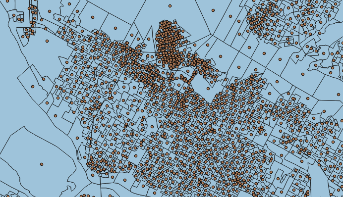
A simple join query looks like this:

EXPLAINANALYZESELECTCount(*)FROMpdJOINptsONST_Intersects(pd.geom,pts.geom);

But the query plan has no parallel elements! Uh oh!

Aggregate  
(cost=222468.56..222468.57 rows=1 width=8) 
(actual time=13830.361..13830.362 rows=1 loops=1)
   ->  Nested Loop  
   (cost=0.28..169725.95 rows=21097041 width=0) 
   (actual time=0.703..13815.008 rows=69534 loops=1)
         ->  Seq Scan on pd  
         (cost=0.00..14271.34 rows=69534 width=2311) 
         (actual time=0.086..90.498 rows=69534 loops=1)
         ->  Index Scan using pts_gix on pts  
         (cost=0.28..2.22 rows=2 width=32) 
         (actual time=0.146..0.189 rows=1 loops=69534)
               Index Cond: (pd.geom && geom)
               Filter: _st_intersects(pd.geom, geom)
               Rows Removed by Filter: 2
 Planning time: 6.348 ms
 Execution time: 13843.946 ms

The plan does involve a nested loop, so there should be an opportunity for parallel join to work magic. Unfortunately no variation of the query or the parallel configuration variables, or the function costs will change the situation: the query refuses to parallelize!

SETparallel_tuple_cost=0.001;SETforce_parallel_mode=on;SETparallel_setup_cost=1;

The ST_Intersects() function is actually a SQL wrapper on top of the && operator and the _ST_Intersects() function, but unwrapping it and using the components directly also has no effect.

EXPLAINANALYZESELECTCount(*)FROMpdJOINptsONpd.geom&&pts.geomAND_ST_Intersects(pd.geom,pts.geom);

The only variant I could get to parallelize omitted the && index operator.

EXPLAINSELECT*FROMpdJOINptsON_ST_Intersects(pd.geom,pts.geom);

Unfortunately without the index operator the query is so inefficient it doesn’t matter that it’s being run in parallel, it will take days to run to completion.

 Gather  
 (cost=1000.00..721919734.88 rows=1611658891 width=2552)
   Number of Workers: 2
   ->  Nested Loop  
   (cost=0.00..576869434.69 rows=1611658891 width=2552)
         Join Filter: _st_intersects(pd.geom, pts.geom)
         ->  Parallel Seq Scan on pd  
         (cost=0.00..13865.73 rows=28972 width=2512)
         ->  Seq Scan on pts  
         (cost=0.00..1275.34 rows=69534 width=40)

So, thus far, parallel query seems to be a wet squib for PostGIS, though I hope with some help from PostgreSQL core we can figure out where the problem lies.

Conclusions

While it is tempting to think “yay, parallelism! all my queries will run $ncores times faster!” in fact parallelism still only applies in a limited number of cases:

• When there is a sequence scan large (costly) enough to be worth parallelizing.
• When there is an aggregate large (costly) enough to be worth parallelizing, and the aggregate function can actually parallize the work effectively.
• (Theoretically) when there is a (nested loop) join large (costly) enough to be worth parallelizing.

Additionally there is still work to be done on PostGIS for optimal use of the parallel features we have available:

• Every function is going to need a cost, and those costs may have to be quite high to signal to the planner that we are not garden variety computations.
• Differences in COST adjustments for different modes need to be explored: why was a 10000 cost needed to kick the aggregation into action, while a 100 cost sufficed for sequence scan?
• Aggregation functions that currently back-load work to the final function may have to be re-thought to do more work in the transfer stage.
• Whatever issue is preventing our joins from parallelizing needs to be tracked down.

All that being said, the potential is to see a large number of queries get $ncores faster, so this promises to be the most important core development we’ve seen since the extension framework arrived back in PostgreSQL 9.1.

Today’s connected enterprise requires a single database that can handle both structured and unstructured data efficiently and that adapts dynamically to swiftly changing data changing and emerging data types. For many organizations, that database is Postgres. With JSON, Postgres can support document databases alongside relational tables and even combine structured and unstructured data.

read more

Recently Robert Haas committed which allows seeing some more detailed information about current wait event of the process. In particular, user will be able to see if process is waiting for heavyweight lock, lightweight lock (either individual or tranche) or buffer pin. The full list of wait events is available in the documentation. Hopefully, it will be more wait events in further releases.

It’s nice to see current wait event of the process, but just one snapshot is not very descriptive and definitely not enough to do any conclusion. But we can use sampling for collecting suitable statistics. This is why I’d like to present pg_wait_sampling which automates gathering sampling statistics of wait events. pg_wait_sampling enables you to gather statistics for graphs like the one below.

Let me explain you how did I draw this graph. pg_wait_sampling samples wait events into two destinations: history and profile. History is an in-memory ring buffer and profile is an in-memory hash table with accumulated statistics. We’re going to use the second one to see insensitivity of wait events over time periods.

At first, let’s create table for accumulated statistics. I’m doing these experiments on my laptop, and for the simplicity this table will live in the instance under monitoring. But note, that such table could live on the another server. I’d even say it’s preferable to place such data to another server.

12345

CREATETABLEprofile_log(tstimestamp,event_typetext,eventtext,countint8);

Secondly, I wrote a function to copy data from pg_wait_sampling_profile view to profile_log table and clean profile data. This function returns number of rows inserted into profile_log table. Also, this function discards pid number and groups data by wait event. And this is not necessary needed to be so.

12345678910111213

CREATEORREPLACEFUNCTIONwrite_profile_log()RETURNSintegerAS<scripttype="math/tex">DECLAREresultinteger;BEGININSERTINTOprofile_logSELECTcurrent_timestamp,event_type,event,SUM(count)FROMpg_wait_sampling_profileWHEREeventISNOTNULLGROUPBYevent_type,event;GETDIAGNOSTICSresult=ROW_COUNT;PERFORMpg_wait_sampling_reset_profile();RETURNresult;END</script>LANGUAGE‘plpgsql’;

And then I run psql session where setup watch of this function. Monitoring of our system is started. For real usage it’s better to schedule this command using cron or something.

1234567891011

smagen@postgres=#SELECTwrite_profile_log();write_profile_log——————-0(1row)</p><p>smagen@postgres=#\watch10FriMar2514:03:092016(every10s)</p><h2id="writeprofilelog">write_profile_log</h2><pre><code>0(1row)

We can see that write_profile_log returns 0. That means we didn’t insert anything to profile_log. And this is right because system is not under load now. Let us create some load using pgbench.

12

$ pgbench -i -s 10 postgres
$ pgbench -j 10 -c 10 -M prepared -T 60 postgres

In the parallel session we can see that write_profile_log starts to insert some data to profile_log table.

12345

FriMar2514:04:192016(every10s)write_profile_log——————-9(1row)

Finally, let’s examine the profile_log table.

12345678910111213

SELECT*FROMprofile_log;ts|event_type|event|count—————————-+—————+——————-+——-2016-03-2514:03:19.286394|Lock|tuple|412016-03-2514:03:19.286394|LWLockTranche|lock_manager|12016-03-2514:03:19.286394|LWLockTranche|buffer_content|682016-03-2514:03:19.286394|LWLockTranche|wal_insert|32016-03-2514:03:19.286394|LWLockNamed|WALWriteLock|682016-03-2514:03:19.286394|Lock|transactionid|3312016-03-2514:03:19.286394|LWLockNamed|ProcArrayLock|82016-03-2514:03:19.286394|LWLockNamed|WALBufMappingLock|52016-03-2514:03:19.286394|LWLockNamed|CLogControlLock|1………………………………………………………………

How to interpret these data? In the first row we can see that count for tuple lock for 14:03:19 is 41. The pg_wait_sampling collector samples wait event every 10 ms while write_profile_log function writes snapshot of profile every 10 s. Thus, it was 1000 samples during this period. Taking into account that it was 10 backends serving pgbench, we can read the first row as “from 14:03:09 to 14:03:19 backends spend about 0.41% of time in waiting for tuple lock”.

That’s it. This blog post shows how you can setup a wait event monitoring of your database using pg_wait_sampling extension with PostgreSQL 9.6. This example was given just for introduction and it is simplified in many ways. But experienced DBAs would easily adopt it for their setups.

P.S. Every monitoring has some overhead. Overhead of wait monitoring was subject of hot debates in mailing lists. This is why features like exposing wait events parameters and measuring each wait event individually are not yet in 9.6. But sampling also has overhead. I hope pg_wait_sampling would be a start point to show on comparison that other approaches are not that bad, and finally we would have something way more advanced for 9.7.

The Postgres-XL 9.5R1Beta2 release went out yesterday. It’s another step forward to have a stable 9.5 release sometime very soon. A few key enhancements from the last beta release are captured in this blog. For the full list, I would recommend to read the release notes.

Support for binary data transfer for JDBC and libpq

If you’d trouble receiving data in binary format via JDBC or libpq, this release should fix those issues for you. The coordinator now have intelligence to figure out if the client is requesting data in binary format and handle those cases correctly.

Pushdown of Append and MergeAppend plans

One of the problems reported with the beta1 release was that for inherited tables, coordinator fails to pushdown plans to the remote nodes even when its possible. A simple example would be:

postgres=# CREATE TABLE parent (a int, b int);
CREATE TABLE
postgres=# CREATE TABLE child1() INHERITS (parent);
CREATE TABLE
postgres=# CREATE TABLE child2() INHERITS (parent);
CREATE TABLE
postgres=# EXPLAIN SELECT sum(a) FROM parent ;
                                                QUERY PLAN                                                
----------------------------------------------------------------------------------------------------------
 Aggregate  (cost=417.19..417.20 rows=1 width=4)
   ->  Append  (cost=100.00..405.89 rows=4521 width=4)
         ->  Remote Subquery Scan on all (datanode_1,datanode_2)  (cost=100.00..100.01 rows=1 width=4)
               ->  Seq Scan on parent  (cost=0.00..0.00 rows=1 width=4)
         ->  Remote Subquery Scan on all (datanode_1,datanode_2)  (cost=100.00..152.94 rows=2260 width=4)
               ->  Seq Scan on child1  (cost=0.00..32.60 rows=2260 width=4)
         ->  Remote Subquery Scan on all (datanode_1,datanode_2)  (cost=100.00..152.94 rows=2260 width=4)
               ->  Seq Scan on child2  (cost=0.00..32.60 rows=2260 width=4)
(8 rows)

You must have noticed that the planner hasn’t chosen the most optimal plan for the query. It would bring all rows from all tables at the coordinator and then perform an aggregation. For very large tables, this will clearly result in bad performance. The new release fixes this problem as seen from the EXPLAIN output below:

postgres=# EXPLAIN SELECT sum(a) FROM parent ;
                                           QUERY PLAN                                            
-------------------------------------------------------------------------------------------------
 Aggregate  (cost=76.50..76.51 rows=1 width=4)
   ->  Remote Subquery Scan on all (datanode_1,datanode_2)  (cost=0.00..65.20 rows=4521 width=4)
         ->  Aggregate  (cost=0.00..65.20 rows=1 width=4)
               ->  Append  (cost=0.00..65.20 rows=4521 width=4)
                     ->  Seq Scan on parent  (cost=0.00..0.00 rows=1 width=4)
                     ->  Seq Scan on child1  (cost=0.00..32.60 rows=2260 width=4)
                     ->  Seq Scan on child2  (cost=0.00..32.60 rows=2260 width=4)
(7 rows)

Partial aggregates will be computed at each node and only the final result is computed on the coordinator. This should improve performance for such queries by many folds.

Process-level control for runtime change in logging level for selective elog() messages

You may remember that in R1Beta1 release we added support for overriding compile time log levels for elog() messages. In this release, that support is further extended to include process-level control for the messages. This will further help the developers and users to investigate issues on a live system. (Note: The server must be compiled with –enable-genmsgids to take benefit of this facility).

The pg_msgmodule_set() and pg_msgmodule_change() functions are used to change the log level of selective elog messages. The following new functions provide a finer control over the logging.

    - pg_msgmodule_enable(pid) - the given pid will start logging as per the
      currently set levels for elog messages.
    
    - pg_msgmodule_disable(pid) - the given pid will stop logging and use the
      compile time levels.
    
    - pg_msgmodule_enable_all(persistent) - all current processes will start
      logging as per currently set levels. If "persistent" is set to true then all
      new processes will also honour the currently set levels.
    
    - pg_msgmodule_disable_all() - all current and future processes will stop
      logging and only use compile time levels.

The latest source code is available at the project website for download. Test the new release and let us know if you find bugs or have suggestions for further improvements.

In my earlier post on new parallel query support coming in PostgreSQL 9.6 I was unable to come up with a parallel join query, despite much kicking and thumping the configuration and query.

It turns out, I didn’t have all the components of my query marked as PARALLEL SAFE, which is required for the planner to attempt a parallel plan. My query was this:

EXPLAINANALYZESELECTCount(*)FROMpdJOINptsONpd.geom&&pts.geomAND_ST_Intersects(pd.geom,pts.geom);

And _ST_Intersects() was marked as safe, but I neglected to mark the function behind the && operator – geometry_overlaps– as safe. With both functions marked as safe, and assigned a hefty function cost of 1000, I get this query:

 Nested Loop  
 (cost=0.28..1264886.46 rows=21097041 width=2552) 
 (actual time=0.119..13876.668 rows=69534 loops=1)
   ->  Seq Scan on pd  
   (cost=0.00..14271.34 rows=69534 width=2512) 
   (actual time=0.018..89.653 rows=69534 loops=1)
   ->  Index Scan using pts_gix on pts  
   (cost=0.28..17.97 rows=2 width=40) 
   (actual time=0.147..0.190 rows=1 loops=69534)
         Index Cond: (pd.geom && geom)
         Filter: _st_intersects(pd.geom, geom)
         Rows Removed by Filter: 2
 Planning time: 8.365 ms
 Execution time: 13885.837 ms

Hey wait! That’s not parallel either!

It turns out that parallel query involves a secret configuration sauce, just like parallel sequence scan and parellel aggregate, and naturally it’s different from the other modes (gah!)

The default parallel_tuple_cost is 0.1. If we reduce that by an order of magnitude, to 0.01, we get this plan instead:

 Gather  
 (cost=1000.28..629194.94 rows=21097041 width=2552) 
 (actual time=0.950..6931.224 rows=69534 loops=1)
   Number of Workers: 3
   ->  Nested Loop  
   (cost=0.28..628194.94 rows=21097041 width=2552) 
   (actual time=0.303..6675.184 rows=17384 loops=4)
         ->  Parallel Seq Scan on pd  
         (cost=0.00..13800.30 rows=22430 width=2512) 
         (actual time=0.045..46.769 rows=17384 loops=4)
         ->  Index Scan using pts_gix on pts  
         (cost=0.28..17.97 rows=2 width=40) 
         (actual time=0.285..0.366 rows=1 loops=69534)
               Index Cond: (pd.geom && geom)
               Filter: _st_intersects(pd.geom, geom)
               Rows Removed by Filter: 2
 Planning time: 8.469 ms
 Execution time: 6945.400 ms

Ta da! A parallel plan, and executing almost twice as fast, just like the doctor ordered.

Complaints

Mostly the parallel support in core “just works” as advertised. PostGIS does need to mark our functions as quite costly, but that’s reasonable since they actually are quite costly. What is not good is the need to tweak the configuration once the functions are properly costed:

• Having to cut parallel_tuple_cost by a factor of 10 for the join case is not any good. No amount of COST increases seemed to have an effect, only changing the core parameter did.
• Having to increase the cost of functions used in aggregates by a factor of 100 over cost of functions used in sequence filters is also not any good.

So, with a few more changes to PostGIS, we are quite close, but the planner for parallel cases needs to make more rational use of function costs before we have achieved parallel processing nirvana for PostGIS.

I’ve been a Postgres DBA since 2005. After all that time, I’ve come to a conclusion that I’m embarrassed I didn’t reach much earlier: Postgres is awful. This isn’t a “straw that broke the camel’s back” kind of situation; there is a litany of ridiculous idiocy in the project that’s, frankly, more than enough to stave off any DBA, end user, or developer. But I’ll limit my list to five, because clickbait.

1. Security Schmecurity

Look, every good Postgres DBA knows that the pg_hba.conf file that handles connection security should have these lines:

local  all  all       trust
host   all  all  all  trust

And then the Postgres developers wonder why it’s so easy to exploit. Here I am, Joe T. Hacker, and I can just do this:

psql -U postgres -h production_server secure_database

And boom! I’m in as the superuser, and I can start dropping tables, replacing tables with whatever I want, screw with data, whatever. Sloppy. Just sloppy.

2. Super Users? Super Losers

Oh yeah, and after I connect to steal sensitive data and then clean up after myself, I can’t even do this:

secure_database=# DROPDATABASE secure_database;
ERROR:  cannot DROP the currently OPENDATABASE 
secure_database=# DROPUSER postgres;
ERROR:  CURRENTUSER cannot be dropped

Ugh! Are you kidding me? This is basic stuff, people. As a superuser, I should be able to circumvent all security, durability, and even internal consistency. That the backend code doesn’t acknowledge what a superuser really is, merely proves that the database owner is just another user. Useless.

Sure, I could use the provided tool and do it from the command line like this:

dropdb -U postgres -h production_server secure_database

But I’m already connected! Oh, or I could switch databases and then do it like this:

secure_database=# \c postgres
secure_database=# DROPDATABASE secure_database;

But if I’ve hacked in, every keystroke counts. It’s not even necessary! They could just queue the action and apply it after I disconnect, right? This kind of amateur work is why I can’t justify being a Postgres DBA anymore.

3. Awkward JOIN Syntax is Awkward

I cut my teeth as a DBA starting in 1999 with Oracle. Now that is a real database engine! One of the really cool things Oracle does is overload the OUTER JOIN syntax with a neat shortcut. Not only is the OUTER decorator optional, but so are LEFT and RIGHT! Let’s compare the only syntax Postgres supports with the snazzy method Oracle provides, and see which one is obviously way better:

-- Postgres (bleh) 
SELECT a.col1, b.col2
  FROM a
  LEFTJOIN b ON(b.a_id = a.id);
 
-- Oracle (Nice!) 
SELECT a.col1, b.col2
  FROM a, b
 WHERE a.id = b.a_id (+);

See that (+) bit? Just slap that on any columns that should join two tables, and it will automatically control how the join works. If it’s on the right, it’s a LEFT JOIN, and if it’s on the left, it’s a RIGHT JOIN. See? Totally intuitive. Sure, Oracle can use the same syntax Postgres childishly demands, but who would purposefully do that? Gross.

4. JSON and the Kitchen Sink

Everyone keeps touting JSON support as some huge benefit to Postgres. Even I did it once or twice. But upon pondering it more seriously, where does it end? What’s the next interface method du jour that we’ll be cobbling onto Postgres next?

First it was XML, then JSON, and next will be what, YAML? They might as well, since you can define your own types anyway.

5. Extensions are the Worst Idea Ever

This is easily the worst of the bunch, and follows naturally from the previous point. Ever since Postgres 9.1, it’s been possible to easily write extensions that are effectively bolted directly to the database engine. Any random schmo can waltz up, whip up some code in basically any language, and it will be able to do any of this. Suddenly Postgres has some “new functionality.”

New functions? New index types? Even override the planner, or fork arbitrary background workers!?

Are you kidding me!? But it gets even worse! There’s a site called PGXN with a related utility for making extensions easy to find and install. I don’t even want to imagine the shenanigans! Any random idiot, including me, could just put an extension there. Just convince a DBA to install it like this:

pgxn install awesome_tool_notanexploitorbotnetiswear

Suddenly they’re pwn3d. Do you want to be pwn3d? I didn’t think so. That’s the kind of risk you run by using Postgres as your primary database engine.

Conclusion

I for one, have seen the light. I can’t believe I was so misled by Postgres for over a decade. How am I even employable at all, having advocated a hacker’s playground for most of my professional career? How can any of us in the Postgres community live with ourselves, knowing we’ve effectively enabled effortless system compromises in the name of functionality?

I guess I’ll go back to using Oracle like the whipped dog I am. It’s what inspired me to be a DBA, and I abandoned it in favor of this travesty. I just pray Larry Ellison will forgive me for my transgressions.

I apologize for everything, and I sincerely hope the rest of the Postgres community joins me in supplication. If our end-users and developers are magnanimous, there might yet be a future for us.

In my Database Hardware Selection Guidelines talk, I emphasized that database servers are usually limited by I/O and memory constraints, not CPU. However, on slide 24 I mentioned one use-case that is CPU-bound — read-only workloads where the working set fits into RAM. Over time, this distinction has gotten more pronounced with the addition of faster I/O (SSDs) and larger-memory systems. What hasn't improved much is CPU speed, though CPU core count has certainly increased.

A subset of CPU-bound workloads are data warehouse queries, where the working set fits into RAM and a large percentage of time is spent in the executor. (The executor runs a state machine, a "plan", created by the optimizer.) This workload distinction is well outlined on slide 5 of a Vitesse DB talk. For queries that spend most of their time in the executor and process data already in RAM, executor overhead is significant.

There were two presentations at the recent PGDay Asia conference that highlight projects designed to reduce executor overhead, leading to massive speedups for specific workloads. The more limited approach was by Kumar Rajeev Rastogi of Huawei. Their approach is to create shared object libraries at table creation time that know about the column structure of each table — this allow specific columns to be accessed rapidly by reducing row access overhead.

Continue Reading »

Someone reported recently on PostGIS mailing list, that they were unable to install PostGIS 2.2.1 bundle or PostGIS 2.2.2 binaries on a clean PostgreSQL 9.5.2 install. Someone also complained about PostgreSQL 9.3 (though not clear the version) if that is a separate issue or the same. I have tested on PostgreSQL 9.5.2 Windows 64-bit and confirmed the issue. The issue does not affect PostgreSQL 9.5.1 and older. I haven't confirmed its an issue with the 32-bit installs, but I suspect so too. This issue will affect OGR_FDW users and people who used our compiled WWW_FDW.

While the last commit fest of PostgreSQL 9.6 is moving to an end with a soon-to-come feature freeze, here is a short story about one of the features that got committed close to the end of it:

commit: 314cbfc5da988eff8998655158f84c9815ecfbcd
author: Robert Haas <rhaas@postgresql.org>
date: Tue, 29 Mar 2016 21:29:49 -0400
Add new replication mode synchronous_commit = 'remote_apply'.

In this mode, the master waits for the transaction to be applied on
the remote side, not just written to disk.  That means that you can
count on a transaction started on the standby to see all commits
previously acknowledged by the master.

To make this work, the standby sends a reply after replaying each
commit record generated with synchronous_commit >= 'remote_apply'.
This introduces a small inefficiency: the extra replies will be sent
even by standbys that aren't the current synchronous standby.  But
previously-existing synchronous_commit levels make no attempt at all
to optimize which replies are sent based on what the primary cares
about, so this is no worse, and at least avoids any extra replies for
people not using the feature at all.

Thomas Munro, reviewed by Michael Paquier and by me.  Some additional
tweaks by me.

Up to 9.5, the GUC parameter synchronous_commit, which defines the way a commit behaves regarding WAL, is able to use the following values:

• ‘on’, the default and safe case where a transaction will wait for its commit WAL record to be written to disk before sending back an acknoledgement to the client. When synchronous_standby_names is used, on top of waiting for the local WAL record to be flushed to disk, the confirmation that the synchronous standby has flushed it as well is waited.
• ‘off’, where no wait is done. So there can be a delay between the moment a transaction is marked as committed and the moment its commit is recorded to disk.
• ‘remote_write’, when synchronous_standby_names is in use, the confirmation from the synchronous standby that the record has been written to storage is waited for. There is no guarantee that the record has been flushed to stable storage though.
• ‘local’, when synchronous_standby_names is in use, process only waits for the flush of the local WAL record to happen locally.

9.6 is going to have a new mode: remote_apply. With this new value, should synchronous_standby_names be in use, not only the flush confirmation of the commit WAL record is waited for, but it is waited that the record has been replayed by the synchronous standby. This simply allows read-balancing consistency, because this way it is guaranteed that a session committing a transaction on a master node will be visible for sessions on the standby once it has been committed locally.

Before this feature, any application willing to do consistent read-balancing across nodes have to juggle with the WAL record of the transaction commit and add some processing at application level to ensure that a record has been applied before ensuring that a given transaction data is visible on a standby node. So this feature is quite a big deal for application relying on read scalability across nodes.

Note that only one synchronous standby can be used with this mode though, hence consistent reads can only be done on two nodes. This limitation may be leveraged with some other features that are still on track for a 9.6 integration, even if the feature freeze is really close by at the moment this post is written:

• Causal reads, which provides a similar way to have balanced reads across nodes, with still the possibility to not see a transaction being visible up to a certain amount of lag. See this thread.
• N-synchronous standbys, which is more simple in itself, because this allows a system to scale from 1 to N synchronous standbys. Things like quorum synchronous standbys are being evaluated as well, with an elegant design. (However note that the more standbys they are, the more the performance penalty when waiting for them with remote_apply). Everything is happening on this thread lately.

However, be careful when using remote_apply. As it interacts with WAL replay, it should not be taken lightly because it could cause performance damages that you would not have imagined first, particularly in case of replay conflicts that could force a standby to wait at replay. This is true for any parameters manipulating how WAL replay behave by the way, another example being recovery_min_apply_delay. If for example this is set to N seconds, a commit on master is sure to take at least this amount of time.

There are many PostgreSQL conference opportunities throughout North America and there are many reasons to attend all of them. There is only one reason you need to attend PgConf.US 2016 and it is not:

• The amazing selection of content to chose from
• The largest networking opportunities available from any PostgreSQL conference
• Rubbing elbows with the who’s who of PostgreSQL
• The dedication to diversity within the community
• The best education opportunities within the PostgreSQL ecosystem

read more

PostgreSQL 9.6 receives suitable support of extensible index access methods. And that’s good news because Postgres was initially designed to support it.

“It is imperative that a user be able to construct new access methods to provide efficient access to instances of nontraditional base types”

Michael Stonebraker, Jeff Anton, Michael Hirohama. Extendability in POSTGRES , IEEE Data Eng. Bull. 10 (2) pp.16-23, 1987

That was a huge work which consists of multiple steps.

1. Rework access method interface so that access method internals are hidden from SQL level to C level. Besides help for custom access methods support, this refactoring is good by itself.
   Committed by Tom Lane.
2. CREATE ACCESS METHOD command which provides legal way for insertion into pg_am with support of dependencies and pg_dump/pg_restore. Committed by Alvaro Herrera.
3. Generic WAL interface which provides custom access methods the way to be WAL-logged. Each built-in access method has its own type of WAL records. But custom access method shouldn’t because it could affect reliability. Generic WAL records represent difference between pages in general way as result of per-byte comparison of original and modified images of the page. For sure, it is not as efficient as own type of WAL records, but there is no choice under restrictions we have. Committed by Teodor Sigaev.
4. Bloom contrib module which is example of custom index access method which uses generic WAL interface. This contrib is essential for testing infrastructure described above. Also, this access method could be useful by itself. Committed by Teodor Sigaev.

I am very thankful for the efforts of committers and reviewers who make it possible to include these features into PostgreSQL.

However, end users don’t really care about this infrastructure. They do care about features we can provide on the base of this infrastructure. Actually, we would be able to have index access methods which are:

• Too hard to add to PostgreSQL core. For instance, we presented fast FTS in 2012. We have 2 of 4 GIN features committed to core. And it seems to be very long way to have rest of features in core. But since 9.6 we would provide it as an extension.
• Not patent free. There are some interesting data structures which are covered by patents (Fractal Tree index, for example). This is why they couldn’t be added to PostgreSQL core. Since 9.6, they could be provided without fork.

Also, I consider this work as an approach (together with FDW) to pluggable storage engines. I will speak about this during my talk at PGCon 2016.

Extremely handy tool for SQL JOINs visualization using Venn diagrams! Must have for all DB people.
SQL Joins visualizer

Source: SQL Joins Visualizer

The new PostgreSQL 9.5 release has a bunch of great features. I describe below the ones I find most interesting.

Upsert

UPSERT is simply a combination of INSERT and UPDATE. This works like this: if a row exists, then update it, if it doesn't exist, create it.

Before Postgres 9.5 when I wanted to insert or update a row, I had to write this:

INSERT INTO test(username, login)
SELECT 'hey', 'ho ho ho'
WHERE NOT EXISTS (SELECT 42 FROM test WHERE username='hey');

UPDATE test SET login='ho ho ho' WHERE username='hey' AND login 
 'ho ho ho';
Which was a little bit problematic. You need to make two queries, and both can have quite complicated WHERE clauses.
In PostgreSQL 9.5 there is much simpler version:
INSERT INTO test(username, login) VALUES ('hey', 'ho ho ho')
ON CONFLICT (username)
DO UPDATE SET login='ho ho ho';
The only requirement is that there should be a UNIQUE constraint on a column which should fail while inserting a row.
The version above makes the UPDATE when the INSERT fails. There is also another form of the UPSERT query, which I used in this blog post.
You can just ignore the INSERT failure:
INSERT INTO test(username, login) VALUES ('hey', 'ho ho ho')
ON CONFLICT (username)
DO NOTHING;
Switching Tables to Logged and Unlogged
PostgreSQL keeps a transaction write ahead log, which helps restore the
  database after a crash, and is used in replication, but it comes with some
  overhead, as additional information must be stored on disk.
In PostgreSQL 9.5 you can simply switch a table from logged to unlogged. The unlogged version can be much faster when filling it with data, processing it etc. However at the end of such operations it might be good to make it a normal logged table. Now it is simple:
ALTER TABLE barfoo SET LOGGED;
JSONB Operators and Functions
This is the binary JSON type, and these new functions allow us to perform
  more operations without having to convert our data first to the slower,
  non-binary JSON alternative.
Now you can remove a key from a JSONB value:
SELECT '{"a": 1, "b": 2, "c": 3}'::jsonb || '{"x": 1, "y": 2, "c": 42}'::jsonb;

     ?column?
──────────────────
 {"b": 2, "c": 3}
And merge JSONB values (the last value's keys overwrit the first's one):
SELECT '{"a": 1, "b": 2, "c": 3}'::jsonb || '{"x": 1, "y": 2, "c": 42}'::jsonb;

                 ?column?
───────────────────────────────────────────
 {"a": 1, "b": 2, "c": 42, "x": 1, "y": 2}
And we have the nice jsonb_pretty() function which instead of this:
SELECT jsonb_set('{"name": "James", "contact": {"phone": "01234 567890",
                   "fax": "01987 543210"}}'::jsonb,
                   '{contact,phone}', '"07900 112233"'::jsonb);

                                   jsonb_set
────────────────────────────────────────────────────────────────────────────────
 {"name": "James", "contact": {"fax": "01987 543210", "phone": "07900 112233"}}
prints this:
SELECT jsonb_set('{"name": "James", "contact": {"phone": "01234 567890",
                   "fax": "01987 543210"}}'::jsonb,
                   '{contact,phone}', '"07900 112233"'::jsonb);


         jsonb_pretty
─────────────────────────────────
  {                              ↵
      "name": "James",           ↵
      "contact": {               ↵
          "fax": "01987 543210", ↵
          "phone": "07900 112233"↵
      }                          ↵
  }
More Information
There are more nice features in the new PostgreSQL 9.5. You can read the full list at https://wiki.postgresql.org/wiki/What'snewinPostgreSQL9.5

PostgreSQL 9.6 has a lot of good features; many of the changes are in the SQL planner, aiming to improve performance by carefully selecting the right execution plan. The great thing here is that doing less work makes many queries much, much faster than they were before.

First, we are now using Foreign Key data in the planner to improve estimates.

Next, we are combining aggregates to avoid duplicating effort.

We’re also improving the way that GROUP BY estimation occurs.

And we’re using partial indexes for index-only scans in more cases.

And we’ve improved estimates for distinct rows, leading to more accurate planning of hash joins and other plan types.

Congratulations to my 2ndQuadrant colleagues Tomas Vondra and David Rowley for their insight, rigour and persistence in chasing down these issues.

All of these things were planned. They didn’t occur randomly, they were part of a coordinated attack on planning problems with big data as part of the AXLE project.

When: 6-8pm Thursday April 21, 2016
Where: Iovation
Who: Eric Ferreira, Database Engineer, Amazon Web Services
What: How to hide a petabyte-scale Data warehouse inside a small OLTP database

You may have heard that Amazon Redshift is a fast, fully managed, petabyte-scale data warehouse. You’ve heard that it’s a shared-nothing cluster architecture, that it scales to hundreds of nodes and terabytes, and that it’s “based on Postgres”. How is that combination possible, and how much of Postgres survived that transformation? Eric Ferreira, who was the first engineer to work on Redshift, will discuss the design, tradeoffs and modifications made to make Redshift the scalable system it is today. Bring your questions!

We will also talk about ways to mix and match Postgres (OLTP) tables and Redshift (DW) tables on a single connection using pgboucer-rr and Postgres external data sources.

Eric started in the database world 26 years ago in Brazil and has implemented most flavors of RDBMS thought his career. He joined Amazon on 2003 and while on AWS/RDS worked on bringing various databases engines into the service. 5 years ago he ventured to start the project that would become Redshift.

—
If you have a job posting or event you would like me to announce at the meeting, please send it along. The deadline for inclusion is 5pm the day before the meeting.
—

Our meeting will be held at Iovation, on the 32nd floor of the US Bancorp Tower at 111 SW 5th (5th & Oak). It’s right on the Green & Yellow Max lines. Underground bike parking is available in the parking garage; outdoors all around the block in the usual spots. No bikes in the office, sorry!

Elevators open at 5:45 and building security closes access to the floor at 6:30.

When you arrive at the Iovation office, please sign in on the iPad at the reception desk.

See you there!