The comprehensive JSON support in PostgreSQL is one of its best-loved features. Many people – particularly those with a stronger background in Javascript programming than in relational databases – use it extensively. However, my experience is that the vast majority of people don’t use it correctly. That causes problems and unhappiness in the long run.
In this article, I will try to point out good and bad uses of JSON in PostgreSQL, and provide you with guidelines that you can follow.
A bad example
This data model exemplifies everything that you can do wrong:
/* this table is fine */
CREATE TABLE people (
   id bigint PRIMARY KEY,
   name text NOT NULL
);

INSERT INTO people VALUES
   (1, 'laurenz'),
   (2, 'julian'),
   (3, 'ants'),
   (4, 'kaarel');

/* this table is ill-defined */
CREATE TABLE rooms (
   id bigint PRIMARY KEY,
   data jsonb
);

INSERT INTO rooms VALUES
   (1,
    '{ "name": "Room 1",
       "reservations": [
           { "who": 1, "from": "2021-06-01 09:00:00", "to": "2021-06-01 10:00:00" },
           { "who": 3, "from": "2021-06-01 10:00:00", "to": "2021-06-01 11:30:00" },
           { "who": 2, "from": "2021-06-01 13:15:00", "to": "2021-06-01 14:45:00" },
           { "who": 1, "from": "2021-06-01 15:00:00", "to": "2021-06-01 16:00:00" }
        ]
     }'),
   (2,
    '{ "name": "Room 2",
       "reservations": [
           { "who": 2, "from": "2021-06-01 09:30:00", "to": "2021-06-01 10:30:00" }
        ]
     }');
First mistake: model regular columns as JSON attributes
There is no reason not to have the room name as a regular column. After all, every room will have a name, and we may want to enforce constraints like uniqueness on the room name.
Second mistake: model tabular data as JSON array
The room reservations are perfectly regular tabular data that define a many-to-many relationship between the rooms and the people. It would have been simple to model the same data with a junction table:
Many people seem to think that storing few large rows in a table is more efficient than storing many small rows. There is some truth to that, since every row has some overhead, and PostgreSQL compresses large data. But if you want to retrieve only parts of the data, or want to modify them, many small rows are much more efficient – as we will see below.
Third mistake: store foreign keys in JSON
The "who" attribute stores a foreign key reference to people. That is not a good idea, because it is impossible for the database to enforce such a constraint: I could just as well have inserted a reference to a non-existing person. With the junction table from above, defining a foreign key is trivial.
Moreover, you often want to join on foreign keys. With JSON, that would require a cross join with the unnested JSON array:
SELECT rooms.data ->> 'name',
       people.name
FROM rooms
   CROSS JOIN LATERAL jsonb_array_elements(
                         rooms.data -> 'reservations'
                      ) AS res(j)
   JOIN people
      ON res.j ->> 'who' = people.id::text;
With the junction table, that would be
SELECT rooms.name,
       people.name
FROM rooms
   JOIN reservations AS r ON r.room_id = rooms.id
   JOIN people ON r.people_id = people.id;
You can probably guess which of these two queries will be more efficient.
Fourth mistake: modify JSON data
If you want to add a new reservation, you have to execute a statement like
UPDATE rooms
SET data = jsonb_set(
              data,
              '{reservations,100000}',
              '{"who": 3, "from": "2021-06-01 11:00:00", "to": "2021-06-01 12:00:00"}',
              TRUE
           )
WHERE id = 2;
This will fetch the complete JSON object, construct a new JSON from it and store that new object in the table. The whole JSON object has to be read and written, which is more I/O than you would want – particularly if the JSON object is large and stored out of line.
Compare how simple the same exercise would be with the junction table:
INSERT INTO reservations VALUES
   (3, 2, '[2021-06-01 11:00:00,2021-06-01 12:00:00)');
This statement will only write a small amount of data.
Deleting a reservation is just as complicated and expensive, and is left as an exercise to the reader.
Fifth mistake: trying to enforce constraints on JSON
So far, our data model offers no protection against overlapping reservations, which would be good to enforce in the database.
With JSON, we are pretty much out of luck here. The best that comes to mind is a constraint trigger, but that would require elaborate locking or the SERIALIZABLE transaction isolation level to be free from race conditions. Also, the code would be far from simple.
With the junction table, the exercise is simple; all we have to do is to add an exclusion constraint that checks for overlaps with the && operator:
CREATE EXTENSION IF NOT EXISTS btree_gist;

ALTER TABLE reservations ADD EXCLUDE USING gist (
   reserved WITH &&,
   room_id WITH =
);
The extension is required to create a GiST index on a bigint column.
Sixth mistake: complicated searches in JSON
Simple searches for equality can be performed with the JSON containment operator @>, and such searches can be supported by a GIN index. But complicated searches are a pain.
Imagine we want to search for all rooms that are occupied at 2021-06-01 15:30:00. With JSON, that would look somewhat like
SELECT id
FROM rooms
   CROSS JOIN LATERAL jsonb_array_elements(
                         rooms.data -> 'reservations'
                      ) AS elem(j)
WHERE CAST(elem.j ->> 'from' AS timestamp) <= TIMESTAMP '2021-06-01 15:30:00'
  AND CAST(elem.j ->> 'to'   AS timestamp) >  TIMESTAMP '2021-06-01 15:30:00';
With our junction table, the query becomes
SELECT room_id
FROM reservations
WHERE reserved @> TIMESTAMP '2021-06-01 15:30:00';
That query can use the GiST index from the exclusion constraint we created above.
If all the above is wrong, should we use JSON in PostgreSQL at all?
Don’t get me wrong: JSON support in PostgreSQL is a wonderful thing. It is just that many people don’t understand how to use it right. For example, the majority of questions about PostgreSQL and JSON asked on Stackoverflow are about problems that arise from the use of JSON where it had better been avoided.
Follow these guidelines when you consider using JSON in PostgreSQL:
Don’t use JSON for data that can easily be stored in database tables.
Avoid large JSON objects if you want to modify individual attributes.
Don’t use JSON if you want to use attributes in complicated WHERE conditions.
Avoid JSON if you want to join on some of the attributes.
Don’t use JSON if you want constraints on the data.
Don’t store references to other tables in JSON attributes.
Often it may be a good idea to store some attributes as regular table columns and others in a JSON. The less you need to process the data inside the database, the better it is to store them as JSON.
A good example
To show an example of how JSON in the database can be used with benefit, let us consider a shop that sells all kinds of mixed goods. There are some properties that all or most of the goods will have, like price, weight, manufacturer, number available or package size. Other attributes may be rare, like the type of power plug, or ambiguous, like the pitch in screws or tuning forks.
Rather than defining a table with hundreds of columns for all the possible attributes, most of which will be NULL, we model the most frequent attributes with normal table columns and use a JSON for the rest:
CREATE TABLE wares (
   id           bigint           PRIMARY KEY,
   name         text             UNIQUE NOT NULL,
   price        numeric(15,2)    NOT NULL,
   weight_kg    double precision NOT NULL,
   available    integer          NOT NULL
      CHECK (available >= 0),
   manufacturer text,
   package_size integer          NOT NULL
      CHECK (package_size >= 0),
   attributes   jsonb
);

/* to search in "attributes" */
CREATE INDEX ON wares USING gin (attributes);

/* for similarity search on "name" */
CREATE EXTENSION IF NOT EXISTS pg_trgm;

CREATE INDEX ON wares USING gin (name gin_trgm_ops);
This will allow efficient queries like
SELECT name, price, available
FROM wares
WHERE name LIKE '%tuning fork%'
  AND attributes @> '{"pitch": "a"}';
Conclusion
There is a lot you can do wrong when using JSON in PostgreSQL, especially if you are not acquainted with relational databases. However, it can be a powerful tool – when used properly.
If you spend any amount of time working with Postgres, it’s likely that at some point you’re going to wonder why it isn’t using an index that you think it should be.
Unlike some databases, you can’t force PostgreSQL to use a specific index, but there are several things you can do to work out what’s going on.
If you’re somewhat new to Postgres, I’m hoping going through these will be interesting, as well as being useful next time you see an issue like this.
I’ll be assuming a basic familiarity with query plans (using EXPLAIN) and Postgres indexing, but honestly not much.
The two main reasons
There are two main categories of reason that result in Postgres not using an index. Either it can’t use the index, or it doesn’t think using the index will be faster.
Working out which of these categories you’re seeing is a great starting point.
Sadly, we can’t tell from a single query plan which case we’re seeing, but through some investigating via multiple query plans, we can work out what’s going on.
Since the reasons that Postgres can’t use an index are more straightforward, and it can be easy to rule out quickly too, I prefer to check that first.
Checking whether Postgres can use the index
There are a few reasons Postgres won’t use a seemingly perfect index for a query.
For example:
A function is preventing its use
A data type mismatch is preventing its use
The index does not exist (oops)
To start with, you can try to disprove you’re in this category of issue by getting a query plan that does use the index.
As I alluded to earlier, some other databases have a “query hints” feature that allows you to (pretty much) force the use of a specific index. But since PostgreSQL does not have such a feature, we can steer clear of that holy war and look at what we can do instead.
For example, Postgres has several parameters that let us temporarily discourage the planner’s choice of certain operations. If you want to encourage an index scan in place of a sequential scan, you can try:
set enable_seqscan = off;
This does not, as the same might suggest, completely disable sequential scans, but rather discourages them by making the planner think they’d be a LOT more expensive than they really would be.
As such, if after setting this to off, this you still get a Seq Scan, there’s a really good chance that Postgres can’t use the index you want, and you’re seeing this category of issue. If, however, it does now use the index you’d hoped, you can skip to the other reasons.
Similarly, if Postgres is picking a different index instead of the index you think would be optimal, then this trick to make indexes invisible shared by Haki Benita (to drop an index and then rollback, all inside a transaction) is a nice way to test this, in a non-production environment of course. Again, whether the query plan changes or not gives you a very good signal as to which category of problem you have.
If Postgres can’t use the index
If you think you’re in the boat of Postgres not being able to use the index, it is first worth checking that the index you’re expecting Postgres to use actually exists (in the environment you’re testing in). If it doesn’t, please believe me that you are not the first, and won’t be the last, to be in this situation! And at least you now have a simple solution.
Assuming the index does exist, though, the next step is to check its definition. This will be helpful for the next two checks we’ll do.
Functions
If your query has a function on the data involved, your index will likely need to match it to get used. For example, a query like:
select * from t where lower(email) = ‘michael@pgmustard.com’;
Won’t use a simple index on “email”, even if in theory it could.
To quickly test if this is the issue you’re seeing, you can request the query plan for the query without the function, for example:
explain select * from t where email = ‘michael@pgmustard.com’;
If you see it is now using your index, and this is how you commonly query that column, you may wish to add a functional index. For example, in this case:
create index i on t (lower(email));
Similarly, you might see this when doing arithmetic on a column. For example, the following query would require an index on “(column + 1)”:
select * from t where column + 1 = 10;
Whereas the equivalent query below would be able to use an index on “column”:
select * from t where column = 10 - 1;
In cases like this, if you are able to change the query, that is normally the better solution.
Datatype mismatches
Earlier, I also mentioned datatype mismatches. You might spot these in the query plan through datatype casting (the :: characters). Postgres can handle some of these without issue, eg varchar to text, but some casts will result in an index not being used.
Here is a contrived example:
explain select * from t where id = 100::numeric;
The explicit cast prevents use of my index, resulting in this query plan:
 Seq Scan on t  (cost=0.00..2041.00 rows=500 width=10)
   Filter: ((id)::numeric = '100'::numeric)
To test whether this is the issue, you can try explicitly casting to the column’s datatype in your query, or avoiding casting being added by the application (eg via an ORM).
If Postgres can use the index, but doesn’t think it will be faster
If you’ve determined that Postgres can use the index, but is choosing not to, then this next section is for you.
There are usually several ways Postgres can get the results of a given query. As such, before executing a query, the planner will estimate the “cost” of different options, and pick the plan with the lowest cost in the hope that it will be the fastest way of executing that query. It’s important to note that these costs are in an arbitrary unit, where higher numbers are a predictor of higher execution times, so it’s the relative numbers that matter, not the absolutes.
As such, if Postgres chooses not to use your index, it is likely that it is calculating the cost of that query plan to be higher than the one it has chosen.
We can verify this by using the tricks mentioned in the previous section, like enable_seqscan = false, or hiding other indexes, and comparing the estimated costs of the different query plans.
The next step is to check whether the execution time of the plan that uses the index is actually faster, or not. You may wish to run it a few times to warm up the cache. If it isn’t faster, you are looking at a case where the planner has correctly chosen not to use your index.
At this point, it is worth noting that the Postgres planner will try to optimize for execution time, rather than efficiency (eg blocks of data read). Although these usually go hand in hand, it is a subtle distinction worth bearing in mind.
There are a few (normally good) reasons for Postgres choosing a sequential scan even when it could use an index scan:
If the table is small
If a large proportion of the rows are being returned
If there is a LIMIT clause and it thinks it can abort early
If none of these are the case, you may wish to skip ahead to the cost estimation section.
If the table is small
If a table is small (very roughly 100 rows or fewer), Postgres may estimate that it will be faster to read the table sequentially and filter out rows as needed, even for highly selective queries.
For example, in pgMustard we show scans on small tables as an anti-tip (scoring 0.0 out of 5.0 for index potential):
If this is a test environment, and you have a lot more data in production, you may need to consider testing on a more realistic dataset.
On the other hand, if this is a realistic dataset already, and it would in fact have been significantly faster to use an index, you may wish to look into the cost constants section below.
If a significant proportion of the rows are being returned
Another case where Postgres will choose to do a sequential scan over an index scan is when a significant proportion of the table is being returned. The exact proportion of what will count as significant will vary depending on the data and cost parameters, but here is an example (with default configuration) of it doing so to return 30% of the data:
Similarly to the small table case, in pgMustard, you will see cases like this as an “index potential” anti-tip, with details about the proportion of rows being returned.
Again, if you work out that (for your query and hardware) it would have been faster to use an index, a good next step is to look into the configuration parameters section below.
Limit clauses
The third case I mentioned above can happen when you have a low LIMIT clause (relative to the total number of rows), and the planner believes it is likely to find enough qualifying rows quickly, allowing it to abort early.
This optimization is a double-edged sword, leading to very fast queries when the planner is correct, and very slow queries when it is wrong. The guide to using EXPLAIN in the PostgreSQL documentation includes a nice LIMIT example, and Christophe Pettus, CEO at PostgreSQL Experts Inc, also succinctly described the potential dangers of using LIMIT in a recent Twitter thread.
As well as avoiding the use of LIMIT when you don’t need it, you can also help the query planner estimate row counts more accurately. Luckily, we’re just about to go into how to do that.
Cost estimation
Naturally, a lot of the times the query planner chooses a suboptimal query plan, it’ll boil down to inaccurate cost estimation.
There are a few ways Postgres can end up badly estimating the overall cost, but the biggest two categories of issue are:
Its row count estimates are way off
Its cost constants are suboptimal
In my experience, bad row count estimates have been the more common of the two, so let’s start there.
Bad row count estimates
The query planner estimates the number of rows each operation will return (mostly) using statistics it has gathered. It keeps these statistics up to date via ANALYZE– not to be confused with the EXPLAIN parameter of the same name.
These estimates can end up way off if the data changes dramatically before it gathers new statistics, or if any of its assumptions are bad for a different reason. Naturally, these bad estimates can affect things that are very important for performance; like join order, join strategy, and of course whether (and how) it uses indexes.
Bad estimates can sometimes be quickly resolved by manually running ANALYZE on the tables involved. If this helps, then you should look into preventing recurrences by ensuring ANALYZE runs more regularly going forwards (eg via autovacuum).
If one of the columns involved has a skewed distribution you may see better estimates after increasing the statistics target.
Another common source of bad estimates is that Postgres assumes that two columns are independent by default. If that’s the root cause, we can ask it to gather data on the correlation between two columns (in the same table, at least) via multivariate statistics.
If this section felt a little rushed, you might like our more in depth post dedicated to bad row count estimates.
Suboptimal configuration
Last, last but certainly not least, we come to planner cost constants. These are used by the query planner to determine the cost of each operation, and subsequently the query plan as a whole.
Cost configuration is a big a topic, so we’ll take a look at the basics and a couple of resources to learn more.
On the topic of index use, if you’re still seeing a Seq Scan instead of the Index Scan that would be faster, then a good parameter to check is random_page_cost:
show random_page_cost;
By default, this is set to 4.0, which is 4x higher than the seq_page_cost of 1.0. This ratio made a lot of sense for spinning disks, but assuming your system has SSDs, you may wish to look into a lower setting. It is not uncommon to see modern PostgreSQL setups with random_page_cost set to 2.0, 1.5, or even 1.1, but as ever, please do test carefully before changing this on production.
To test whether it helps, you can change a parameter like this in a session and rerun EXPLAIN to see whether they result in a different query plan being chosen.
Another common cost-related reason for Postgres favouring a Seq Scan over an Index Scan is if it is parallelizing operations. To quickly test this, you can disable parallel execution locally and re-request the query plan, for example via:
set max_parallel_workers_per_gather = 0;
There are many other cost-related configuration parameters that you may find beneficial to tune. The query planning section of the PostgreSQL docs contains a useful list, and you can then look up each of them on the postgresqlco.nf website, which includes advice, courtesy of Josh Berkus’ excellent annotated.conf, as well as useful information and links courtesy of the team at Ongres.
In summary
So in summary, our first step was to check whether Postgres could use the index.
If it couldn’t, we double-checked it actually existed, before seeing whether a function or datatype mismatch could be the problem.
If it could, we compared the execution time to make sure it wasn’t right all along, then looked into the row count estimates and planner cost constants, looking for ways to help it calculate the relative costs more accurately.
Next steps
If, after this, you’re still facing an issue, both the PostgreSQL Wiki and Stack Overflow have good guides for troubleshooting performance problems, asking for help, and reporting bugs.
I hope it’s been somewhat helpful though, and it’d be great to hear from you either way. I’d particularly welcome hearing about things I could improve, for clarity or completeness.
If you’d like a monthly email with Postgres performance blog posts and videos, as well as any pgMustard news, check out our newsletter.
In the last installment of the pipeline blog series, we explored writing streaming JSON data into PostgreSQL using Kafka Connect. In this blog, it’s time to find out if our fears of encountering mutant monsters in the gloom of an abandoned uranium mine were warranted or not.
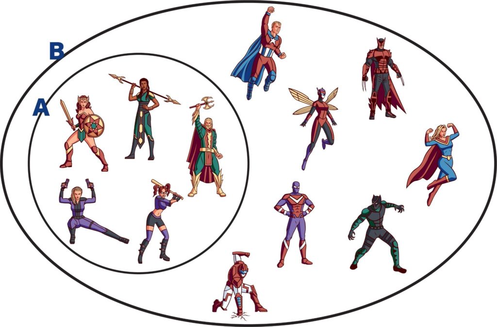
Or perhaps it could be related to a mathematical superset? B is a superset of A if B contains all the elements of A (B ⊇ A). For example, if A is the set of all superheroes that use weapons, and B is the set of all superheroes, then B is the superset of A:
However, my guess is that the mathematical idea inspired Apache Superset as the project page proclaims that:
“Apache Superset is a modern data exploration and visualization platform that is fast, lightweight, intuitive, and loaded with options that make it easy for users of all skill sets to explore and visualize their data, from simple line charts to highly detailed geospatial charts.”
Here are some interesting points I discovered about Superset:
It is based on SQL and can connect to any SQL database that is supported by SQL Alchemy. So at least in theory, this gives good interoperability with a large number of data sources (but also excludes some common NoSQL databases, unfortunately).
But what if you aren’t an SQL guru? It supports a zero-code visualization builder, but also a more detailed SQL Editor.
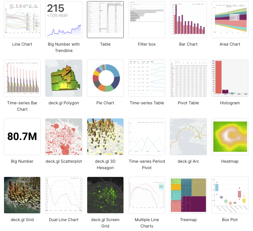
Superset supports more than 50 built-in charts offering plenty of choices for how you visualize your data.
The main Superset concepts are databases, data sources, charts, and dashboards.
Superset started out in Airbnb, and graduated to being a top-level Apache project this year (2021), so it’s timely to be evaluating it now.
In this blog, I wanted to get Apache Superset working with PostgreSQL. Some of the challenges I expected were:
How easy is it to deploy Apache Superset?
Can Apache Superset be connected to PostgreSQL (specifically, a managed Instaclustr PostgreSQL service, I had access to a preview service)?
Is it possible to chart JSONB column data types in Apache Superset?
Does Apache Superset have appropriate chart types to display the basic NOAA tidal data and also map the locations?
2. Deploying Apache Superset
So far in the pipeline series I’ve been used to the ease of spinning up managed services on the Instaclustr platform (e.g. Elasticsearch and Kibana). However, we currently don’t have Superset on our platform, so I was going to have to install and run it on my laptop (a Mac). I’m also used to the ease of deploying Java-based applications (get a jar, run jar). However, Superset is written in Python, which I have no prior experience with. I, therefore, tried two approaches to deploying it.
Approach 1
I initially tried to install Superset from scratch using “pip install apache-superset”. However, this failed with too many errors.
Approach 2
My second approach used Docker, which eventually (it was very slow to build) worked. I just used the built-in Mac Docker environment which worked fine—but don’t forget to increase the available memory from the default of 2GB (which soon fails) to at least 6GB. It’s also very resource-hungry while running, using 50% of the available CPU.
Superset runs in a browser at http://localhost:8088
Don’t forget to change the default user/password from admin/admin to something else.
So, given our initial false start, and by using Docker, it was relatively easy to deploy and run Superset.
3. Connecting Superset to PostgreSQL
In Superset, if you go into “Data->Databases” you find that there’s already a PostgreSQL database and drivers installed and running in the Docker version. It turns out that Superset uses PostgreSQL as the default metadata store (and for the examples).
But I wanted to use an external PostgreSQL database, and that was easy to configure on Superset following this documentation.
Superset has the concepts of databases and datasets. After connecting to the Instaclustr managed PostgreSQL database and testing the connection you “Add” it, and then a new database will appear. After configuring a database you can add a dataset, by selecting a database, schema, and table.
So, the second challenge was also easy, and we are now connected to the external PostgreSQL database.
4. Apache Superset Visualization Types
Clicking on a new dataset takes you to the Chart Builder, which allows you to select the visualization type, select the time (x-axis) column (including time grain and range), and modify the query. By default, this is the “Explore” view which is the zero-code chart builder. There’s also the SQL Lab option which allows you to view and modify the SQL query.
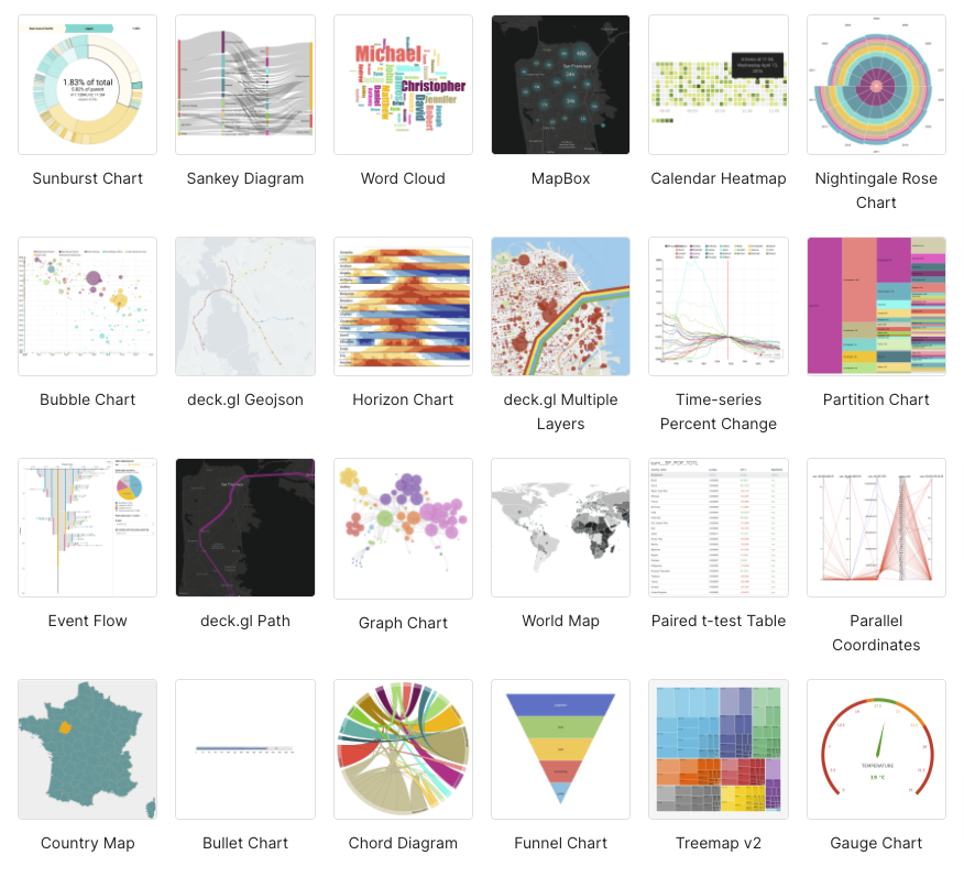
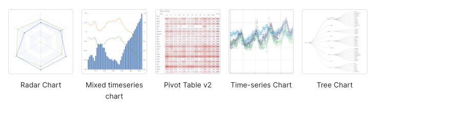
Here are the available visualization types available (which I noticed includes my favorite graph type, the Sankey diagram, which is great for systems performance analysis; Chord diagrams are also cool):
6. Charting PostgreSQL Column Data With Apache Superset
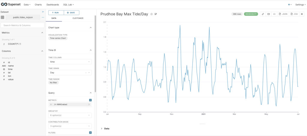
Next, I wanted to check that I could actually get data out of PostgreSQL and chart it, so I cheated (a bit) and uploaded a year’s worth of NOAA tidal data for one location using the CSV option (“Data->Upload a CSV”), which creates a table with columns in PostgreSQL, and a new corresponding dataset in Superset. From the new dataset, I created a Time-series Chart, with time as the x-axis, Day as the Time Grain, and MAX(value) as the metric. This gives the following graph showing the maximum tide height per day, so that ticks another box.
7. Charting PostgreSQL JSONB Data With Apache Superset
The real challenge was to chart the NOAA data that was streaming into my PostgreSQL database as a result of the previous blog, and which was being stored as a JSONB data type.
I created a dataset for the NOAA JSON table and tried creating a chart. Unfortunately, the automatic query builder interface didn’t have any success interpreting the JSONB data type, it just thought it was a String. So after some Googling, I found a workaround involving “virtual” datasets (JSON or Virtual datasets don’t seem to feature in the Apache documentation, unfortunately).
However, if you look at “Data->Datasets” you’ll notice that each dataset has a Type, either Physical or Virtual. Datasets are Physical by default, but you can create Virtual datasets in the SQL Lab Editor. Basically, this allows you to write your own SQL resulting in a new “virtual” table/dataset. What I needed to do was to create a SQL query that reads from the NOAA JSONB data type table and creates a new table with the columns that I need for charting, including (initially at least) the station name, time, and value.
Here’s an example of the JSON NOAA data structure:
Again, after further googling and reading my blog on PostgreSQL JSON, and testing it out in the SQL Editor (you can see the results), I came up with the following SQL that did the trick:
SELECT
cast(d.item_object->>'t' as timestamp) AS __timestamp, json_object->'metadata'->'name' AS name, AVG(cast(d.item_object->>'v' as FLOAT)) AS v
FROM
tides_jsonb,jsonb_array_elements(json_object->'data')
with ordinality d(item_object, position)
where d.position=1
GROUP BY name, __timestamp;
Compared with the previous approach using Elasticsearch, this SQL achieves something similar to the custom mapping I used which overrides the default data type mappings. The difference is that using PostgreSQL you have to manually extract the correct JSON elements for each desired output column (using the “->>” and “->” operators), and cast them to the desired types. The functions “jsonb_array_elements” and “ordinality” are required to extract the first (and only) element from the ‘data’ array (into d), which is used to get the ‘v’ and ‘t’ fields.
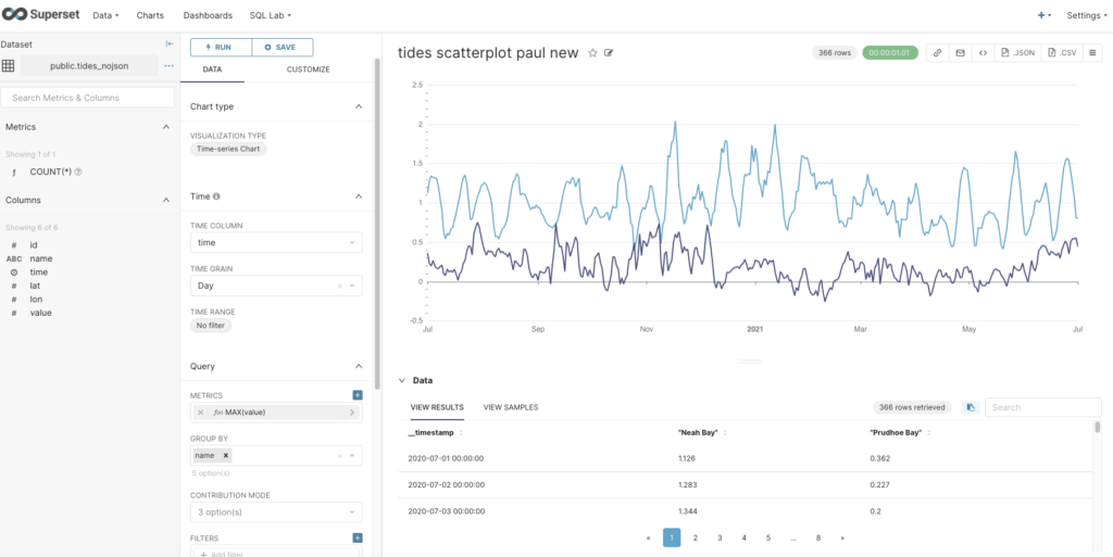
Once you’ve got this working, you click on the Explore button and “Save or Overwrite Dataset” to save the query as a virtual dataset. The new dataset (with Type Virtual in the Datasets view) is now visible, and you can create a Time-series Chart for it just as we did with the sample (CSV) column table. To display multiple graphs on one chart you also have to Group by name. The (automatically generated) SQL is pretty complex, but I noticed that it’s just nesting the above virtual query in a “FROM” clause to get the virtual dataset and graph it.
Here’s the chart with data from 2 stations:
So far, so good, now let’s tackle the mapping task.
8. Mapping PostgreSQL JSONB Data
The final task I had set myself was to attempt to replicate displaying station locations on a map, which I’d previously succeeded in doing with Elasticsearch and Kibana.
The prerequisite is to add the lat/lon JSON elements to a virtual dataset as follows:
SELECT
cast(d.item_object->>'t' as timestamp) AS __timestamp, json_object->'metadata'->'name' AS name,
cast(json_object->'metadata'->>'lat' as FLOAT) AS lat,
cast(json_object->'metadata'->>'lon' as FLOAT) AS lon,
AVG(cast(d.item_object->>'v' as FLOAT)) AS v
FROM
tides_jsonb,jsonb_array_elements(json_object->'data')
with ordinality d(item_object, position)
where d.position=1
GROUP BY name, __timestamp, lat, lon
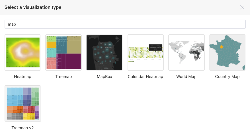
The next step is to find a map visualization type. Typing “map” into the visualization type search box gives these results:
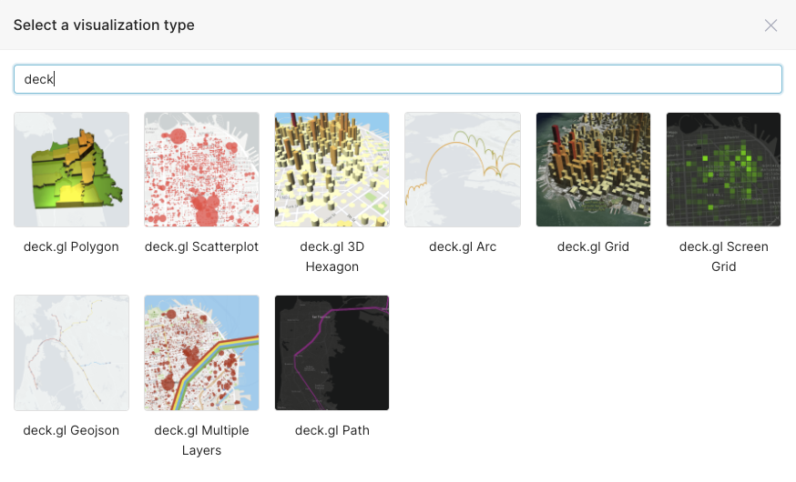
As you can see, only a few of these are actual location-based maps, and they turned out to be mainly maps for country data. I also searched for “geo” and found one map called “deck.gl Geojson”, which looked more hopeful, and searching for “deck” I found a bunch of potential candidates:
I found out that deck.gl is a framework for detailed geospatial charts so these looked promising. However, after trying a few I discovered that they didn’t have any base maps displayed. After some frantic googling, I also discovered that you need a “Mapbox” token to get them to work. You can get a free one from here. To apply the Mapbox token you have to stop the Superset Docker, go to the Superset/Docker folder, edit the non-dev config file (.env-non-dev) and add a line “MAPBOX_API_KEY = “magic number”, save it, and start superset docker again—and then the base maps will appear.
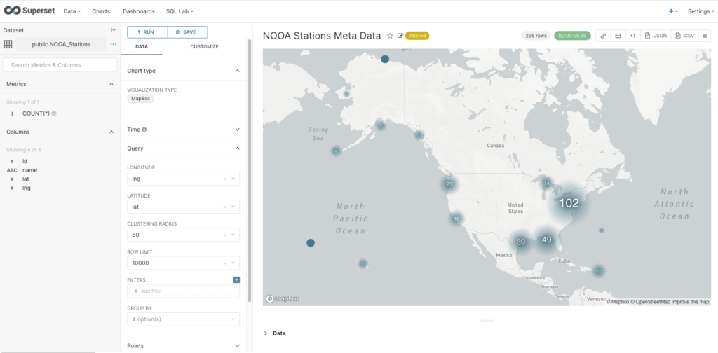
The final problem was selecting an appropriate chart type. This turned out to be trickier than I thought, as many of them have specific use cases (e.g. some automatically aggregate or cluster points). For example, the MapBox visualization successfully shows the location of the NOAA tidal stations, but at the zoomed-out level, it aggregates them and displays a count. Note that for map charts, you have to select the Longitude and Latitude columns; but watch out as this is the reverse order to the normal lat/lon order convention.
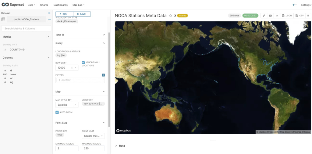
Finally the deck.gl Scatterplot visualization type (with satellite map style) succeeded in showing the location of each station (small blue dots around coastline).
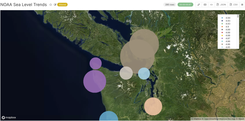
But what I really wanted to do was show a tidal value for each station location as I’d done with Kibana previously. Luckily I worked out that you can also change the size and color of the points as well. I uploaded the NOAA sea level trends (mm/year), configured point size to be based on the value with a multiplier of 10 to make them bigger, and selected Point Color->Adaptative formatting, which changes the point color based on the point size metric (unfortunately the colour gradient isn’t meaningful). Zooming in on the map you can see what this looks like in more detail, and you can easily see which tidal stations have bigger sea level trends (maybe best not to buy coastal properties there!)
9. Conclusions
How does the PostgreSQL+Superset approach compare with the previous Elasticsearch+Kibana approach?
The main difference I noticed in using them was that in Elasticsearch the JSON processing is performed at indexing time with custom mappings, whereas for Superset the transformation is done at a query-time using SQL and JSONB operators to create a virtual dataset.
In terms of interoperability, Kibana is limited to use with Elasticsearch, and Superset can be used with any SQL database (and possibly with Elasticsearch, although I haven’t tried this yet). Superset has more chart types than Kibana, although Kibana has multiple plugins (which may not be open source and/or work with Open Distro/OpenSearch).
There may also be scalability differences between the two approaches. For example, I encountered a few scalability “speed-humps” with Elasticsearch, so a performance comparison may be interesting in the future.
Follow the Pipeline Series
Part 1: Building a Real-Time Tide Data Processing Pipeline: Using Apache Kafka, Kafka Connect, Elasticsearch, and Kibana
Part 2: Building a Real-Time Tide Data Processing Pipeline: Using Apache Kafka, Kafka Connect, Elasticsearch, and Kibana
Part 3: Getting to Know Apache Camel Kafka Connectors
Part 4: Monitoring Kafka Connect Pipeline Metrics with Prometheus
Part 5: Scaling Kafka Connect Streaming Data Processing
Part 6: Streaming JSON Data Into PostgreSQL Using Open Source Kafka Sink Connectors
Part 7: Using Apache Superset to Visualize PostgreSQL JSON Data
I have seen a people comparing YugabyteDB and PostgreSQL, and surprised by the different throughput when running a simple test on a from a single session. The purpose of a distributed database is to scale out. When running on a single node without the need for High-Availability-without-data-loss (this is a tautology), a monolith database will always perform with lower latency. Because a distributed DB is designed to ensure the persistence (the D in ACID) though RPC (remote procedure calls) rather than local writes.
Here is a simple workload:
drop table if exists demo;
create table demo(
 i int primary key,
 t timestamp default clock_timestamp()
);

\timing on

do $$
 begin
  truncate demo;
  for i in 1..1e4 loop
   insert into demo(i) values(i);
   commit;
  end loop;
 end;
$$;

select
 count(*)/extract(epoch from max(t)-min(t)) "rows/s",
 count(*),max(t)-min(t) "duration"
 from demo;
YugabyteDB
Here is the run in the current production (stable) release, a RF=3 with all nodes on the same VM (for this test, in order to be independent on network latency, you don't do that in production):
[postgres@yb0 ~]$ psql -p 5433

yugabyt=# select version();
                                                  version
------------------------------------------------------------------------------------------------------------
 PostgreSQL 11.2-YB-2.6.1.0-b0 on x86_64-pc-linux-gnu, compiled by gcc (Homebrew gcc 5.5.0_4) 5.5.0, 64-bit

yugabyte=# do $$ begin truncate demo; for i in 1..1e4 loop insert into demo(i) values(i); commit; end loop; end; $$;
DO
Time: 37130.036 ms (00:37.130)

yugabyte=# select count(*)/extract(epoch from max(t)-min(t)) "rows/s",count(*),max(t)-min(t) "duration" from demo;

      rows/s      | count |    duration
------------------+-------+-----------------
 270.115078207229 | 10000 | 00:00:37.021258
The number by itself is not important. It is a lab on one VM but I'll run everything in the same machine to compare the thoughput.
[postgres@yb0 ~]$ psql -p 5432

postgres=# select version();

                                                version
-------------------------------------------------------------------------------------------------------------
 PostgreSQL 13.4 on x86_64-pc-linux-gnu, compiled by gcc (GCC) 8.4.1 20200928 (Red Hat 8.4.1-1), 64-bit

postgres=# do $$ begin truncate demo; for i in 1..1e4 loop insert into demo(i) values(i); commit; end loop; end; $$;
DO
Time: 5533.086 ms (00:05.533)

postgres=# select count(*)/extract(epoch from max(t)-min(t)) "rows/s",count(*),max(t)-min(t) "duration" from demo;

       rows/s       | count |    duration
-------------------------+-------+-----------------
 1809.0359900474075 | 10000 | 00:00:05.527806
This is what make you think that PostgreSQL is faster. Yes there is a 1:7 factor here in transactions per second.
But we are comparing apples and oranges in term of resilience. YugabyteDB was running with Replication Factor RF=3 so that each write is propagated to a quorum of 2 out of 3 replicas. In a Yugabyte cluster with RF=3, you can kill a node and:
2/3 of reads and writes continue to operate as if nothing happens. Thanks to the sharding of tables into tablets.
1/3 of reads and writes, those which had their leader on the dead node, have to wait a few seconds to get one of the followers, on the surviving nodes, to be elected new leader (Raft protocol)
And all continues because we have the quorum. And all is consistent. And no committed transaction has been lost. The only consequence is that, until the first node is back, or a new node added, loosing a second node will stop the database. Still with no data loss. But RF=3 can tolerate only one node down, by definition.
This protection involves remote procedure calls. Let's see how PostgreSQL would behave with some higher availability
PostgreSQL with standby
I'll add two standby databases to my PostgreSQL cluster:
Those are two asynchronous standbys receiving the streamed WAL.
I run the same mini-workload:
postgres=# do $$ begin truncate demo; for i in 1..1e4 loop insert into demo(i) values(i); commit; end loop; end; $$;
select count(*)/extract(epoch from max(t)-min(t)) "rows/s",count(*),max(t)-min(t) "duration" from demo;
DO
Time: 6437.456 ms (00:06.437)

postgres=# select count(*)/extract(epoch from max(t)-min(t)) "rows/s",count(*),max(t)-min(t) "duration" from demo;

       rows/s       | count |    duration
-------------------------+-------+-----------------
 1554.5772428235664 | 10000 | 00:00:06.432617
This is still quite fast. But is this High Availability? Not at all. Yes in case of total failure of the primary database, I don't need to restore a backup and can failover to one of the standby databases. But:
I'll lose some committed transactions because I'm in ASYNC replication. Recovery Point Objective is RPO>0
Because of the preceding, this cannot be automated. You need a human decision to evaluate the risk of data loss, and the probability to get the failed primary site back at least to get the WAL with the latest transactions, before opening the standby. Human decision means, in practice, a Recovery Time Objective in minutes or hours: RTO>0
This cannot be compared with YugabyteDB replication where all is automated within seconds, without data loss.
PostgreSQL with synchronous standby
We can reduce the RPO with synchronous replication:
postgres=# do $$ begin truncate demo; for i in 1..1e4 loop insert into demo(i) values(i); commit; end loop; end; $$;
DO
Time: 13613.487 ms (00:13.613)

postgres=# select count(*)/extract(epoch from max(t)-min(t)) "rows/s",count(*),max(t)-min(t) "duration" from demo;

      rows/s      | count |    duration
-----------------------+-------+-----------------
 734.861683966413 | 10000 | 00:00:13.608003
The throughput has been divided by two.
Are we in High Availability here? This SYNC configuration requires complex monitoring and management. Because, even in sync, the persistence of WAL does not happen at the same time: first written and (fsync'd) then send (and acknowledged) to the standby, then returning "commit successful" to the user. There is no two-phase commit here. This is very different, in case of failure, from a consensus protocol as we can find in a distributed database. PostgreSQL databases are often used with ASYNC, and this is a very good DR (Disaster Recovery) solution where the data loss is minimal after a manual failover. SYNC replication is possible, but doesn't qualify as the same High Availability than distributed databases.
The numbers are not important here. They will depend on your machine and your network. Distributed databases can be in sync in a multi-AZ cluster, even multi-region. The point is that the thoughput is lower for a single session. But, because all nodes are active, this scales-out when having multiple sessions load-balanced over all nodes. You cannot do that with PostgreSQL standby that are read only.
YugabyteDB scale-out
I'm adding a "j" column for job number in my table:
drop table if exists demo;
create table demo(
 j int, i int,
 t timestamp default clock_timestamp(),
 primary key(j,i)
);
And run 3 parallel jobs doing the same inserts:
for i in {0..2} ; do
psql -h yb$i -p 5433 -c 'do $$ begin for i in 1..1e4 loop insert into demo(j,i) values('$i',i); commit; end loop; end; $$ ; ' &
done ; wait
With my 3 concurrent sessions I have inserted at 550 transaction per second. Again, this is a small lab. While single session short transaction have limited rate because of the distributed nature of commits, it can scale to many nodes. If you stay on one VM without synchronous replication to another site, PostgreSQL will be faster. Where distributed databases show all their power is when you add nodes, for high availability and load balance, without adding complexity because all the distributed protocol is already there.
There are additional things that you can't see in this short test. PostgreSQL cannot sustain those inserts indefinitely. The shared buffers are filling, checkpoint will occur, the filesystem cache will be synced to disk. And the most important: at some point you will need to VACUUM the table before the transaction id wraps around, or the database will hang. The first minutes of insert are very optimistic in PostgreSQL, which is fine with short peaks of activity.
Note that I've written something similar in the past about RDS PostgreSQL vs. Aurora. Even if both cannot scale out the writes, the HA in Aurora relies on remote WAL sync.
To many parameters to consider? Don't panic. Because YugabyteDB has the same API as PostgreSQL - it uses the same SQL and PL/pgSQL layer and similar open source license - you are not locked in your initial decision. You can start with PostgreSQL and scale with YugabyteDB, or vice-versa.
I released new significant version of plpgsql_check - plpgsql_check 2.0.1. Although there are only two new features (and few bugfixes), these two features are important. I wrote about benefits of plpgsql_check for PL/pgSQL language developers in my blog Why you need plpgsql_check (if you write procedures in PLpgSQL). The plpgsql_check is PostgreSQL extensions, that does static analyze of PL/pgSQL code. It can detect lot of possible runtime bugs before execution, it can detect some performance or security isues too. More plpgsql_check can do coverage analyze, and has integrated profiler and tracer. The PL/pgSQL language is relative static type strict language, and then the static analyze is working well. But there are two limits. The statis analyze cannot to work with objects and values that are created (calculated) at runtime. These objects are local temporary tables (PostgreSQL doesn't support global temporary tables yet) and the results of dynamic SQL:
postgres=# \sf+ fx1
        CREATE OR REPLACE FUNCTION public.fx1(tablename text)
         RETURNS void
         LANGUAGE plpgsql
1       AS $function$
2       DECLARE r record;
3       BEGIN
4         EXECUTE format('SELECT * FROM %I', tablename) INTO r;
5         RAISE NOTICE 'id=%', r.id;
6       END;
7       $function$

postgres=# SELECT * FROM plpgsql_check_function('fx1');
┌──────────────────────────────────────────────────────────────────────────────────────┐
│                                plpgsql_check_function                                │
╞══════════════════════════════════════════════════════════════════════════════════════╡
│ warning:00000:4:EXECUTE:cannot determinate a result of dynamic SQL                   │
│ Detail: There is a risk of related false alarms.                                     │
│ Hint: Don't use dynamic SQL and record type together, when you would check function. │
│ error:55000:5:RAISE:record "r" is not assigned yet                                   │
│ Detail: The tuple structure of a not-yet-assigned record is indeterminate.           │
│ Context: SQL expression "r.id"                                                       │
└──────────────────────────────────────────────────────────────────────────────────────┘
(6 rows)

postgres=# \sf+ fx2
        CREATE OR REPLACE FUNCTION public.fx2()
         RETURNS void
         LANGUAGE plpgsql
1       AS $function$
2       BEGIN
3         CREATE TEMP TABLE IF NOT EXISTS ltt(a int);
4         DELETE FROM ltt;
5         INSERT INTO ltt VALUES(10);
6       END;
7       $function$

postgres=# SELECT * FROM plpgsql_check_function('fx2');
┌───────────────────────────────────────────────────────────┐
│                  plpgsql_check_function                   │
╞═══════════════════════════════════════════════════════════╡
│ error:42P01:4:SQL statement:relation "ltt" does not exist │
│ Query: DELETE FROM ltt                                    │
│ --                 ^                                      │
└───────────────────────────────────────────────────────────┘
(3 rows)
In plpgsql_check 2.0.0 I can use pragmas TYPE and TABLE (note: an syntax of pragma in plpgsql_check is little bit strange, because the language PL/pgSQL doesn't support native syntax for pragma (custom compiler directive) (like ADA language or PL/SQL language):
CREATE OR REPLACE FUNCTION public.fx1(tablename text) RETURNS void LANGUAGE plpgsql 1 AS $function$ 2 DECLARE r record; 3 BEGIN 4 PERFORM plpgsql_check_pragma('TYPE: r (id int)'); 5 EXECUTE format('SELECT * FROM %I', tablename) INTO r; 6 RAISE NOTICE 'id=%', r.id; 7 END; 8 $function$
postgres=# \sf+ fx2 CREATE OR REPLACE FUNCTION public.fx2() RETURNS void LANGUAGE plpgsql 1 AS $function$ 2 BEGIN 3 CREATE TEMP TABLE IF NOT EXISTS ltt(a int); 4 PERFORM plpgsql_check_pragma('TABLE: ltt (a int)'); 5 DELETE FROM ltt; 6 INSERT INTO ltt VALUES(10); 7 END; 8 $function$
Fast load into a database table is a feature we need on any database. Datawarehouses use it daily. OLTP requires it regularly. And probably from the beginning of their existence to migrate data to it. With Python,the psycopg2 client is commonly used and I'll start there (this is the first post in a series). The main motivation is that psycopg2 doesn't have prepared statements, and parsing each INSERT, even with a list of rows, is not efficient for loading million of rows. But it has a nice alternative as it can call the COPY command.
All this works on any PostgreSQL-compatible engine. I'll use YugabyteDB here because loading data involves multiple nodes, and it is then critical to do it right. I'll simulate an IoT ingest taking the function from the Database performance comparison for IoT use cases. This project uses INSERT ... VALUES to load data but I'll use COPY which is the most efficient for any PostgreSQL compatible database that supports it. I've submitted a PR with some optimizations (now merged).
I'll define the IoT events with dataclasses_json and will use the psychopg2 driver which is the most frequently used with Python. This requires:
pip install psycopg2 dataclasses_json
I re-use the generate_events code from the MaibornWolff project:
The only thing I changed here is define a timestamp datatype rather than an epoch.
I create an iot_demo table to store those events:
importpsycopg2yb=psycopg2.connect('postgres://yugabyte:franck@yb1.pachot.net:5433/yugabyte')yb.cursor().execute("""
        drop table if exists iot_demo;
        create table if not exists iot_demo (
            timestamp timestamp,
            device_id text,
            sequence_number bigint,
            temperature real,
            primary key(device_id,timestamp,sequence_number)
            );
""")
This connects to my very small Yugabyte database that I keep publicly open. You can easily create one following the documentation or our free tier cloud.
I have defined the primary key without mentioning HASH or RANGE partitioning so that the code is compatible with any PostgreSQL database. In YugabyteDB, the defaults are HASH for the first column in the primary key and ASC for the others, so what I want to achieve is: hash sharding to distribute the devices and range on time to get the measures together.
As generate_events is a generator (there's a yield clause to return the event in the loop) I just loop on it to build a string version of the events (tab-separated columns)
In psychopg2 the copy_from() reads from a file, but here I generate events into an in-memory StringIO that will be read like a file by copy_from(). Don't forget to seek(0) after writing to it so that copy_from()starts at the begining. And truncate(0)when done.
I'm keeping all simple there. If there are some character strings that contain tabs or newlines, you may have to handle them as with TSV format. But in a future post I'll show that you can do better.
Pandas
You can also use pandas to format the CSV correctly and use copy_expert which allows for more options:
importpandasimportpsycopg2defload_events_with_copy_from_psycopg2(device_id,num_events):yb=psycopg2.connect('postgres://yugabyte:franck@yb1.pachot.net:5433/yugabyte')ysql=yb.cursor()ysql.execute("set yb_default_copy_from_rows_per_transaction=1000")events=[]foreventingenerate_events(device_id=device_id,start_timestamp=0,num_events=num_events,sequence_number=1,device_spread=1):events.append(event)csv=io.StringIO(pandas.DataFrame(events).to_csv(header=True,index=False))ysql.copy_expert("""
        COPY iot_demo(timestamp,device_id,sequence_number,temperature)
        FROM STDIN WITH DELIMITER ',' CSV HEADER
        """,csv)yb.commit()ysql.close()
The one with pandas is easier, as it takes care of the CSV format.
Threads
A distributed database scales and you may load from multiple threads. This is easy as psycopg2 is thread safe.
Here is the main program that loads events in loops in threads:
The goal of this post was to show that even with this old psycopg2 driver that doesn't support prepared statements, we can do fast loads. I'll write more on bulk inserts. In PostgreSQL, as in YugabyteDB, COPY is the optimal way to ingest data. The difference is that PostgreSQL by default loads all data in one transaction, and you can define intermediate commits with ROWS_PER_TRANSACTION option. However, in YugabyteDB, the inserted rows have to be buffered to be distributed efficiently to the tablet servers. It is more efficient to limit the size of transactions and the yb_default_copy_from_rows_per_transaction has been introduced with a default value of 1000 to avoid memory issues when loading large files on small servers. Setting this to 0 reverts to the same as PostgreSQL in case you want to be sure that all is rolled back in case of failure.
Nowadays it is becoming more frequent for systems and applications to require querying data from outside the main database. PostgreSQL supports querying external postgres data using two core extensions dblink and postgres-fdw , the last one is a Foreign Data Wrapper (FDW), that is an implementation of SQL/MED standard, which is part of ANSI SQL 2003 standard specification. FDW is widely recommended to be used in PostgreSQL for this activity instead of dblink, because it provides standards-compliant syntax for accessing remote tables/data, and can give us better performance in some cases.
Executing queries that need external data can sometimes be slow but PostgreSQL’s planner can apply some optimizations for this, such as: running some activity in the remote server to try to reduce the data transferred from there or if it is possible execute remote JOIN operations to take advantage of remote server resources. In addition, it is possible to make adjustments to help the planner choose better decisions and help the executor take advantage of this. This blog will show the reader some simple tips, examples, and explanations about how to increase performance of queries using FDW in PostgreSQL.
Improving from the definition
Normally when working with FDW it is necessary to define three types of objects, such as: a SERVER to establish the connections to the remote host, the USER that defines what user will access the external host and finally the FOREIGN TABLE to map the tables in the foreign server. All of these objects mentioned previously have some options that can help to improve the performance of queries.
1: Fetch_size
The FDW retrieves data from the remote server using row bunches and the size of these bunches is defined by the fetch_size option (default 100). This option can be specified for a SERVER or FOREIGN TABLE, and the values defined for the last one have priority.
Example :
CREATE SERVER pgserver FOREIGNDATA WRAPPER postgres_fdw  OPTIONS(host'localhost', port '5432',dbname 'db2');
  CREATEUSER MAPPING FORcurrent_user  SERVER pgserver   OPTIONS (user'postgres',password 'my_pass');
CREATEFOREIGNTABLE f_tables.customers (
	customerid int4  ,
	firstname varchar(50) ,
	lastname varchar(50) ,
	username varchar(50) ,
	age int2 ,
	gender varchar(1)
) SERVER pgserver OPTIONS (schema_name'public', table_name'customers');
And if executes EXPLAIN command to see what is happening with the query is possible see how the executor implements Remote SQL:
[18580] postgres@db1 LOG:  execute<unnamed>: explain (analyze,verbose) select o.*,ftc.firstname from orders o join f_tables.customers as ftc using (customerid)
[22696] postgres@db2 LOG:  statement: STARTTRANSACTIONISOLATIONLEVELREPEATABLEREAD
[22696] postgres@db2 LOG:  execute<unnamed>: DECLARE c1 CURSORFORSELECT customerid, firstname FROMpublic.customers
[22696] postgres@db2 LOG:  statement: FETCH10000FROM c1
...until20000
[22696] postgres@db2 LOG:  statement: CLOSE c1
[22696] postgres@db2 LOG:  statement: COMMITTRANSACTION
Obviously, the transaction will require fewer Fetch operations to get all data, this will translate in less time executing the query, as the EXPLAIN output shows us. So if is necessary to process a large number of rows from FDW please take this option into consideration.
2: Extensions
The PostgreSQL planner can decide if any WHERE operations could be executed on a remote host as long as it is safe to do so, in this case only WHERE clauses using built-in functions are considered safe, but the extensions option can help us to define our own functions and operators as safe (packaged in extension form) and this will indicate to the PostgreSQL’s planner that it is safe to execute WHERE operations on the remote host and this will translate into a better performance. For this, it is necessary to package the functions in an extension way and set them as IMMUTABLE. This option can only be specified for SERVER objects.
For example:
EXPLAIN (analyze,verbose) select o.*,ftc.firstname from orders o join f_tables.customers as ftc using (customerid)  where super_age(ftc.age)

    Hash Join  (cost=470.00..642.84rows=249 width=148) (actual time=18.702..59.381rows=525 loops=1)
  Output: o.orderid, o.orderdate, o.customerid, o.netamount, o.tax, o.totalamount, ftc.firstname
  Hash Cond: (ftc.customerid = o.customerid)
  ->Foreign Scan on f_tables.customers ftc  (cost=100.00..268.48rows=187 width=122) (actual time=14.233..54.635rows=842 loops=1)
        Output: ftc.customerid, ftc.firstname, ftc.lastname…
        Filter: super_age((ftc.age)::integer)
        Rows Removed by Filter: 19158
        Remote SQL: SELECT customerid, firstname, age FROMpublic.customers
  ->  Hash  (cost=220.00..220.00rows=12000 width=30) (actual time=4.282..4.282rows=12000 loops=1)
        Output: o.orderid, o.orderdate, o.customerid, o.netamount, o.tax, o.totalamount
        Buckets: 16384  Batches: 1  Memory Usage: 889kB
        ->  Seq Scan onpublic.orders o  (cost=0.00..220.00rows=12000 width=30) (actual time=0.022..1.659rows=12000 loops=1)
              Output: o.orderid, o.orderdate, o.customerid, o.netamount, o.tax, o.totalamount
Planning Time: 0.197 ms
Execution Time: 60.013 ms
In this case, if the function super_age is packaged as an extension and sets the name to the extension option the result changes
CREATE EXTENSION fdw_functions; -- the extension must be loaded in both server (origin and remote)
ALTER SERVER pgserver  OPTIONS (extensions 'fdw_functions');
    Hash Join  (cost=470.00..635.36rows=249 width=148) (actual time=39.761..39.985rows=525 loops=1)
  Output: o.orderid, o.orderdate, o.customerid, o.netamount, o.tax, o.totalamount, ftc.firstname
  Hash Cond: (ftc.customerid = o.customerid)
  ->Foreign Scan on f_tables.customers ftc  (cost=100.00..261.00rows=187 width=122) (actual time=37.855..37.891rows=842 loops=1)
        Output: ftc.customerid, ftc.firstname, ftc.lastname…
        Remote SQL: SELECT customerid, firstname FROMpublic.customers WHERE (public.super_age(age))
  ->  Hash  (cost=220.00..220.00rows=12000 width=30) (actual time=1.891..1.892rows=12000 loops=1)
        Output: o.orderid, o.orderdate, o.customerid, o.netamount, o.tax, o.totalamount
        Buckets: 16384  Batches: 1  Memory Usage: 889kB
        ->  Seq Scan onpublic.orders o  (cost=0.00..220.00rows=12000 width=30) (actual time=0.009..0.842rows=12000 loops=1)
              Output: o.orderid, o.orderdate, o.customerid, o.netamount, o.tax, o.totalamount
Planning Time: 0.162 ms
Execution Time: 40.364 ms
Therefore if it is necessary to filter some data in the WHERE clause using its own function, bear in mind this option provided by FDW.
3: Use_remote_estimate
PostgreSQL’s planner decides which is the better strategy to execute the queries, this decision is based on the table’s statistics, so, if the statistics are outdated the planner will choose a bad execution strategy. Autovacuum process will help to keep statistics updated, but does not execute ANALYZE commands on foreign tables, hence to keep statistics updated on foreign tables it is necessary to run manually ANALYZE on those tables. To avoid outdated statistics, the FDW has an option to get the statistics from the remote server on the fly, this option is precisely use_remote_estimate and can be specified for a foreign table or a foreign server.
[18580] postgres@db1 LOG:  execute<unnamed>: explain (analyze,verbose) select o.*,ftc.firstname from orders o join f_tables.customers as ftc using (customerid)   where gender ='F'
[22696] postgres@db2 LOG:  statement: STARTTRANSACTIONISOLATIONLEVELREPEATABLEREAD
[22696] postgres@db2 LOG:  statement: EXPLAINSELECT customerid, firstname FROMpublic.customers WHERE ((gender ='F'::text))
[22696] postgres@db2 LOG:  statement: EXPLAINSELECT customerid, firstname FROMpublic.customers WHERE ((gender ='F'::text)) ORDERBY customerid ASC NULLS LAST
[22696] postgres@db2 LOG:  statement: EXPLAINSELECT customerid, firstname FROMpublic.customers WHERE ((((SELECTnull::integer)::integer) = customerid)) AND ((gender ='F'::text))
[22696] postgres@db2 LOG:  execute<unnamed>: DECLARE c1 CURSORFORSELECT customerid, firstname FROMpublic.customers WHERE ((gender ='F'::text))
[22696] postgres@db2 LOG:  statement: FETCH10000FROM c1
[22696] postgres@db2 LOG:  statement: FETCH10000FROM c1
[22696] postgres@db2 LOG:  statement: CLOSE c1
[22696] postgres@db2 LOG:  statement: COMMITTRANSACTION
As shown in the logs, many EXPLAIN commands are thrown to the remote server and obviously the planning time will increase, but the planner gets better statistics to decide which is the better execution plan, which translates into better execution times.
Pool
Another improvement could be using a pooling solution, like pgbouncer, with static connections for FDWs. This would reduce the overhead of establishing new connections each time is required. Benchmarks about the benefits of using pgBouncer can be found: here and there. If you want to test FDW with pgbouncer by yourself you can use this labs or you can check the results of this test here, where it is possible to see the positive impact of using a pgbouncer for pooling the FDW connections .
Conclusions
The tips and examples shown above have shown us that sometimes with minimum changes if we are using FDW in our queries in PostgreSQL we can get some reasonable performance benefits. Of course you must analyze if each tip fixes your data scenery. In new PostgreSQL’s releases, it is possible that new options will appear to boost our queries with FDW. If you know any other tips about FDW performance, please feel free to share them with us.
Supporting PostgreSQL DBAs is an important part of daily life here atCrunchy Data. I’ve recently run across a few use cases where utility queries based on the current state of the database are needed. A simple example could be where you have a table that is the target of logical replication and theidcolumn becomes out of sync with the sequence that generated the data. This would result in new rows having primary key conflicts. To correct this issue, you would need to set the sequence to generate values past the current max value in the table.
This example is part of a larger class of problems which are best solved with functionality that SQL by itself does not directly provide: Dynamic DDL.Data Definition Language(DDL) in SQL itself is notoriously non-dynamic, with strict parsing rules, predefined data types, table structures, and queries based on known and articulated columns.
So how can we bend SQL to our will and execute Dynamic DDL Postgres queries without having to manually write these queries each time? In this next installment of my Devious SQL series (see posts #1 and #2), I’ll show you some SQL approaches to get the job done.
Altering sequence restart values
Let us again consider a scenario where we want to explicitly provide theRESTARTvalue for asequencevia a query. This is an easy thing to express in terms of what we would like to do: we want to reset a sequence to start after the current maximum value of the table it is associated with.
Trying the naïve approach, we get:
ALTER SEQUENCE big_table_id_seq RESTART (SELECT max(id) + 1 FROM big_table);
ERROR:  syntax error at or near "(", at character 41
STATEMENT:  ALTER SEQUENCE big_table_id_seq RESTART (SELECT max(id) + 1 FROM big_table);
As we can see, this approach isn't supported by the PostgreSQL grammar, as it is expecting an actual value here, not a subquery (as nice as that would be).
So what are some approaches here?
Usingpsqlvariable substitution
If we are usingpsql, we have a few options on how to solve this problem. One approach is usingpsqlvariablesand first selecting the value we want into a variable, then substituting this value into the expression we pass to psql:
-- use \gset to set a psql variable with the results of this query
SELECT max(id) + 1 as big_table_max from big_table \gset
-- substitute the variable in a new query
ALTER SEQUENCE big_table_id_seq RESTART :big_table_max ;
ALTER SEQUENCE
In this example, we are using the\gsetcommand to capture the results of the first query and store it for use later in thepsqlsession. We then interpolate this variable into our expression using the:big_table_maxsyntax, which will be passed directly to the PostgreSQL server.
Usingpsql's\gexeccommand
Another method of utilizingpsqlfor dynamic SQL is constructing the query as aSELECTstatement returning the statements you wish to run, then using the\gexeccommand to execute the underlying queries. First let's look at making ourselves a query that returns the statement we want, then we'll run this statement using\gexec:
SELECT 'ALTER SEQUENCE big_table_id_seq RESTART ' || max(id) + 1 as query FROM big_table;
SELECT 'ALTER SEQUENCE big_table_id_seq RESTART ' || max(id) + 1 as query FROM big_table \gexec
query
ALTER SEQUENCE big_table_id_seq RESTART 100001
ALTER SEQUENCE
A benefit of this approach compared to the variable substitution one is that this can work with more complex statements and multiple return values, so you could construct queries based on arbitrary conditions and generate more than one SQL query; the first implementation is limited to queries that return single rows at a time. This also gives you a preview of the underlying SQL statement that you will be runningbeforeyou execute it against the server with\gexec, so provides some level of safety if you were doing some sort of destructive action in the query.
Dynamic SQL withoutpsql
Not everyone usespsqlas the interface to PostgreSQL, despite its obvious superiority :-), so are there ways to support dynamic SQL using only server-side tools? As it so happens there are several, using basically the same approach of writing aplpgsqlsnippet to generate the query, thenEXECUTEto run the underlying utility statement. These roughly correlate to the approaches in thepsqlsection above in that they work best for single or multiple dynamic statements.
DOblocks
To use server-side Dynamic SQL we will need to construct our queries usingplpgsqland execute the underlying text as if we were issuing the underlying query ourselves.
DO $$
BEGIN
    EXECUTE format('ALTER SEQUENCE big_table_id_seq RESTART %s', (SELECT max(id) + 1 FROM big_table));
END
$$
LANGUAGE plpgsql;
DO
In this case we are using PostgreSQL's built-informat()function which substitutes arguments similar toprintf()in C-based languages. This allows us to interpolate the subquery result we were wanting in this case, resulting in a string that PostgreSQL canEXECUTEand giving us the result we want.
Create anexec()function
Almost identical in function to theDOblock, we can also create a simpleplpgsqlfunction that simply callsEXECUTEon it input parameter like so:
CREATE OR REPLACE FUNCTION exec(raw_query text) RETURNS text AS $$
BEGIN
  EXECUTE raw_query;
  RETURN raw_query;
END
$$
LANGUAGE plpgsql;

SELECT exec(format('ALTER SEQUENCE big_table_id_seq RESTART %s', (SELECT max(id) + 1 FROM big_table)));
CREATE FUNCTION
exec
ALTER SEQUENCE big_table_id_seq RESTART 100001
This may seem like a fairly pointless change compared to the previous approach, as we have basically only moved our query into a parameter that we pass in, but what it buys us is the ability to call this function against a list of queries that we construct using normal SQL, giving us the option of running each in turn.
Restrictions
So what type of SQL can be run in each of these sorts of approaches, and are there any restrictions in what we can run via Dynamic SQL with these methods? The main consideration about the different approaches is related to commands that need to be run outside of an explicit transaction block.
Consider if we wanted to run aREINDEX CONCURRENTLYon all known indexes, so we used theexec()approach to construct aREINDEX CONCURRENTLYstatement for all indexes in thepublicschema:
SELECT
    exec(format('REINDEX INDEX CONCURRENTLY %I', relname))
FROM
    pg_class
JOIN
    pg_namespace
ON pg_class.relnamespace = pg_namespace.oid
WHERE
    relkind = 'i' AND
    nspname = 'public'
ERROR:  REINDEX CONCURRENTLY cannot be executed from a function
CONTEXT:  SQL statement "REINDEX INDEX CONCURRENTLY big_table_pkey"
PL/pgSQL function exec(text) line 3 at EXECUTE
As you can see here, this won't work as a function due toREINDEX CONCURRENTLYneeding to manage its own transaction state; in PostgreSQL, functions inherently run inside a transaction to allow the impact of a function to either completely succeed or completely fail. (Atomicity in ACID.)
Let's try this using\gexec:
SELECT
    format('REINDEX INDEX CONCURRENTLY %I', relname)
FROM
    pg_class
JOIN
    pg_namespace
ON pg_class.relnamespace = pg_namespace.oid
WHERE
    relkind = 'i' AND
    nspname = 'public'
\gexec
REINDEX
Since the\gexechandling is done bypsql, the resulting statement is effectively run at the top-level as if it appeared literally in the SQL file.
More advanced usage
Look for a followup blog article where I go into more advanced techniques using Dynamic SQL, particularly using the\gexecfunction orexec()itself. Until next time, stay devious1!
Footnotes:
1Devious: longer and less direct than the most straightforward way.
Most database tables have an artificial numeric primary key, and that number is usually generated automatically using a sequence. I wrote about auto-generated primary keys in some detail in a previous article. Occasionally, gaps in these primary key sequences can occur – which might come as a surprise to you.
This article shows the causes of sequence gaps, demonstrates the unexpected fact that sequences can even jump backwards, and gives an example of how to build a gapless sequence.
Gaps in sequences caused by rollback
We are used to the atomic behavior of database transactions: when PostgreSQL rolls a transaction back, all its effects are undone. As the documentation tells us, that is not the case for sequence values:
To avoid blocking concurrent transactions that obtain numbers from the same sequence, a nextval operation is never rolled back; that is, once a value has been fetched it is considered used and will not be returned again. This is true even if the surrounding transaction later aborts, or if the calling query ends up not using the value. For example an INSERT with an ON CONFLICT clause will compute the to-be-inserted tuple, including doing any required nextval calls, before detecting any conflict that would cause it to follow the ON CONFLICT rule instead. Such cases will leave unused “holes” in the sequence of assigned values.
This little example shows how a gap forms in a sequence:
CREATE TABLE be_positive (
   id bigint GENERATED ALWAYS AS IDENTITY PRIMARY KEY,
   value integer CHECK (value > 0)
);

-- the identity column is backed by a sequence:
SELECT pg_get_serial_sequence('be_positive', 'id');

   pg_get_serial_sequence
════════════════════════════
 laurenz.be_positive_id_seq
(1 row)

INSERT INTO be_positive (value) VALUES (42);
INSERT 0 1

INSERT INTO be_positive (value) VALUES (-99);
ERROR:  new row for relation "be_positive" violates
        check constraint "be_positive_value_check"
DETAIL:  Failing row contains (2, -99).

INSERT INTO be_positive (value) VALUES (314);
INSERT 0 1

TABLE be_positive;

 id │ value
════╪═══════
  1 │    42
  3 │   314
(2 rows)
The second statement was rolled back, but the sequence value 2 is not, forming a gap.
This intentional behavior is necessary for good performance. After all, a sequence should not be the bottleneck for a workload consisting of many INSERTs, so it has to perform well. Rolling back sequence values would reduce concurrency and complicate processing.
Gaps in sequences caused by caching
Even though nextval is cheap, a sequence could still be a bottleneck in a highly concurrent workload. To work around that, you can define a sequence with a CACHE clause greater than 1. Then the first call to nextval in a database session will actually fetch that many sequence values in a single operation. Subsequent calls to nextval use those cached values, and there is no need to access the sequence.
As a consequence, these cached sequence values get lost when the database session ends, leading to gaps:
As with all other objects, changes to sequences are logged to WAL, so that recovery can restore the state from a backup or after a crash. Since writing WAL impacts performance, not each call to nextval will log to WAL. Rather, the first call logs a value 32 numbers ahead of the current value, and the next 32 calls to nextval don’t log anything. That means that after recovering from a crash, the sequence may have skipped some values.
To demonstrate, I’ll use a little PL/Python function that crashes the server by sending a KILL signal to the current process:
CREATE FUNCTION seppuku() RETURNS void
   LANGUAGE plpython3u AS
'import os, signal
os.kill(os.getpid(), signal.SIGKILL)';
Now let’s see this in action:
CREATE SEQUENCE seq;

SELECT nextval('seq');

 nextval
═════════
       1
(1 row)

SELECT seppuku();
server closed the connection unexpectedly
	This probably means the server terminated abnormally
	before or while processing the request.
Upon reconnect, we find that some values are missing:
It is a little-known fact that sequences can also jump backwards. A backwards jump can happen if the WAL record that logs the advancement of the sequence value has not yet been persisted to disk. Why? Because the transaction that contained the call to nextval has not yet committed:
CREATE SEQUENCE seq;

BEGIN;

SELECT nextval('seq');

 nextval
═════════
       1
(1 row)

SELECT nextval('seq');

 nextval
═════════
       2
(1 row)

SELECT nextval('seq');

 nextval
═════════
       3
(1 row)

SELECT seppuku();
psql:seq.sql:9: server closed the connection unexpectedly
	This probably means the server terminated abnormally
	before or while processing the request.
This looks scary, but no damage can happen to the database: since the transaction didn’t commit, it was rolled back, along with all possible data modifications that used the “lost” sequence values.
However, that leads to an interesting conclusion: don’t use sequence values from an uncommitted transaction outside that transaction.
How to build a gapless sequence
First off: think twice before you decide to build a gapless sequence. It will serialize all transactions that use that “sequence”. That will deteriorate your data modification performance considerably.
You almost never need a gapless sequence. Usually, it is good enough if you know the order of the rows, for example from the current timestamp at the time the row was inserted. Then you can use the row_number window function to calculate the gapless ordering while you query the data:
SELECT created_ts,
       value,
       row_number() OVER (ORDER BY created_ts) AS gapless_seq
FROM mytable;
You can implement a truly gapless sequence using a “singleton” table:
CREATE TABLE seq (id bigint NOT NULL);

INSERT INTO seq (id) VALUES (0);

CREATE FUNCTION next_val() RETURNS bigint
   LANGUAGE sql AS
'UPDATE seq SET id = id + 1 RETURNING id';
It is important not to create an index on the table, so that you can get HOT updates– and so that the table does not get bloated.
Calling the next_val function will lock the table row until the end of the transaction, so keep all transactions that use it short.
Conclusion
I’ve shown you several different ways to make a sequence skip values — sometimes even backwards. But that is never a problem, if all you need are unique primary key values.
Resist the temptation to try for a “gapless sequence”. You can get it, but the performance impact is high.
If you are interested in learning about advanced techniques to enforce integrity, check out our blogpost on constraints over multiple rows.
In Part 6 and Part 7 of the pipeline series we took a different path in the pipe/tunnel and explored PostgreSQL and Apache Superset, mainly from a functional perspective—how can you get JSON data into PostgreSQL from Kafka Connect, and what does it look like in Superset. In Part 8, we ran some initial load tests and found out how the capacity of the original Elasticsearch pipeline compared with the PostgreSQL variant. These results were surprising (PostgreSQL 41,000 inserts/s vs. Elasticsearch 1,800 inserts/s), so in true “MythBusters” style we had another attempt to make them more comparable.
Explosions were common on the TV show “MythBusters”! (Source: Shutterstock)
1. Apples-to-Oranges Comparison
Next, I tried the classic “Myth Busters” second attempt methodology: just make it work! For this approach I discarded the Kafka Connect Elasticsearch sink connector and used an Elasticsearch client (The OpenSearch Python Client) directly to generate the load into Kafka (okay, this is really more like “Apples-to-weirdest fruit you can think of” comparison at this point). This client supports the security plugin, but I did have to modify it to send my example JSON tidal data, and to use the Bulk API to index multiple documents at a time.
The results were definitely better this time around:
First, using the non-Bulk API, the maximum capacity was 5,000 index operations a second (with 60 client processes, and 50% Elasticsearch data nodes CPU utilization).
Second, using the Bulk API the maximum capacity increased to a more comparable 37,500 index operations a second (50 client processes, 80% Elasticsearch data nodes CPU, 16% master nodes CPU)
Here’s what the Elasticsearch results look like. It’s apparent that using the Bulk API makes the biggest difference, probably because the HTTP protocol is much slower than the index operation.
The results of the “just make it work” apples-to-oranges attempt between the PostgreSQL and Elasticsearch pipelines are now very comparable (well within a typical 10% experimental error margin), at around 40,000 inserts/s:
Now, 40,000 inserts/s translates to an impressive 3.4 billion inserts per day, way more than we would need for our example NOAA tidal data pipeline. Doing some back-of-the-envelope calculations, we have a maximum of 500 NOAA tidal stations, with 10 metrics each, refreshing every 6 minutes, so we only need 14 inserts/s. However, if the scope of our pipeline increases, say to all the NOAA land-based weather stations (30,000, and there are even more stations in the ocean and air, etc.), which have on average of say 10 metrics, and say a refresh rate every 10 seconds, then the load is a more demanding 30,500 inserts/s. Both of the prototype pipeline sink systems would cope with this load (although I haven’t taken into account the extra load on the Kafka connect cluster, due to the Kafka source connectors). This is a good example of “scalability creep”—it’s always a good idea to plan for future growth in advance.
2. Comparing Elasticsearch and PostgreSQL Replication Settings
Given my relative lack of knowledge about PostgreSQL (which is okay as we have lots of PostgreSQL experts available due to the recent acquisition of Credativ, I wondered if the replication settings for PostgreSQL were really comparable with Elasticsearch.
Elasticsearch uses synchronous replication—each index operation succeeds only after writing to the primary, and (concurrently) every replica also acknowledges it. As far as I can tell, this only happens after the write request is both written to Lucene (into memory) and to the disk log. This achieves both high durability and consistency, and the data can be immediately read from the replicas.
Here’s what I found out about PostgreSQL replication.
First, to confirm if synchronous replication is enabled (it is enabled on the Instaclustr managed PostgreSQL service, as long as you request more than 1 node at creation time), use a PostgreSQL client (e.g. psql), connect to the cluster, and run:
SHOW synchronous_commit
this will be on, and
SHOW synchronous_standby_names
which will show 1 or more node names,
depending on how many nodes you specified at cluster creation – e.g. if 2 nodes, then there will be 1 name, if 3 nodes, then there will be 2 names
Second, “on” is the default commit mode, but there are more possibilities. Multiple options are available and include master-only or master and replicas, durability, and consistency. Here’s my summary table:
synchronous_ commit
Commit ack when
Master durability
Replica durability
Replica consistency
Lag (increasing)
off
master only acks (in memory)
F
F
F
0
local
master only flush (to disk)
T
F
F
1
remote_write
replicas ack (in memory)
T
F
F
2
on (default)
replicas flush (to disk)
T
T
F
3
remote_apply
replicas applied (available for reads)
T
T
T
4
The off and local modes provide no replication, whereas the rest do. All modes except off provide master durability (in the case of server failure, the data is persisted), but only on and remote_apply provide replica durability. Finally, remote_apply is the only option that also provides replica read consistency, as the data is made available for reads before the ack is sent. Note that for remote_write the data will eventually be written to disk (assuming the server hasn’t crashed – 200ms is the default time for flushes), and for remote_apply, the data will be made available for reads, but it’s just done asynchronously.
Each option will take longer to acknowledge and will in theory, therefore, reduce the throughput of the system. This also seems to be the case in practice as shown in this graph ( results normalized to best-case off mode):
The remote_apply mode is indeed the worst case for performance, with exactly half of the throughput of the fastest off mode. So, why is this relevant for the pipeline comparison? Well, the PostgreSQL results were obtained using the default on mode. However, a more directly comparable mode, in terms of durability and consistency, is the remote_apply mode. However, in practice the performance difference between remote_apply and on is small (only about 4%) so the results are good enough for a rough comparison.
To get these results, I also had to find out how to set the scope of the settings correctly. This is because synchronous_commit can be set at the scope of transactions, sessions, users, databases, and instances (here’s a good blog to read) so I set it at the user level as follows:
ALTER USER username SET synchronous_commit=remote_apply;
Finally, I was curious to see what the lags were for my running system. The best way I could find to see this was using this command:
select * from pg_stat_replication;
This returns information including write_lag (corresponding to remote_write delay), flush_lag (remote_flush delay), and replay_lag (remote_apply delay), along with the sync_state of the server (which is useful confirmation that it’s working as expected). See this documentation for an explanation of the metrics. This confirmed that the replication was keeping up (which was logical as the CPU utilization on the replica server was minimal).
3. Result Caveats
(Source: Shutterstock)
Given the apples-to-dragon fruit (the oddest fruit that I actually like) nature of these results, here are a few caveats to take into account:
Replication for both Elasticsearch and PostgreSQL was “2” (i.e. 1 primary copy of data and 1 replica copy). The impact of increasing this to a recommended “3” was not measured.
The PostgreSQL synchronous_commit modes can have a big impact on throughput, and you should check if the default value of “on” meets your requirements for performance, durability, consistency, and availability (which I didn’t mention above, but there is another setting to control how many replicas must reply before a commit. With 1 replica these won’t have any impact, but with more replicas they may).
Not being able to push the PostgreSQL master CPU higher than 50% was surprising, and suggests either hardware or software settings bottlenecks (this may also be related to the database connections).
The PostgreSQL results were obtained using our internal managed PostgreSQL preview service which had not yet been fully optimized for performance. The public preview (recently announced) and GA releases are likely to be more highly tuned.
Elasticsearch scales horizontally with more nodes and shards, and PostgreSQL scales vertically with larger server sizes. I didn’t try further scaling for this comparison.
The comparison used different types of sink system clients, so it really isn’t on a level playing field:
The PostgreSQL client was a Kafka Connect sink connector but had potential issues with database pooling and leaks, so it’s unlikely that it had the optimal number of database connections
The Elasticsearch client was a customized Python client due to issues with the security plug-in and lack of Bulk API support in my Kafka sink connector
In theory, PostgreSQL could benefit from the equivalent to the Elasticsearch Bulk API (e.g. multirow inserts perhaps), but I didn’t try it, but I don’t expect it to have as much impact as the Elasticsearch Bulk API, given that the PostgreSQL message-based TCP/IP protocol is likely more efficient than HTTP
However, the identical JSON example data was used for both alternatives, the cluster sizes and costs are very similar, and the results are, perhaps unexpectedly, very similar. Anyway, my goal wasn’t really to “race” them against each other, but rather to get a feel for the likely throughput and to confirm that they were both sensible choices for a pipeline. So far so good!
In the next and final blog of this series, we’ll sum up and evaluate the technologies from multiple perspectives.
Follow the Pipeline Series
Part 1: Building a Real-Time Tide Data Processing Pipeline Part 1
Part 2: Building a Real-Time Tide Data Processing Pipeline Part 2
Part 3: Getting to Know Apache Camel Kafka Connectors
Part 4: Monitoring Kafka Connect Pipeline Metrics with Prometheus
Part 5: Scaling Kafka Connect Streaming Data Processing
Part 6: Streaming JSON Data Into PostgreSQL Using Open Source Kafka Sink Connectors
Part 7: Using Apache Superset to Visualize PostgreSQL JSON Data
Part 8: Kafka Connect Elasticsearch vs. PostgreSQL Pipelines: Initial Performance Results
Part9: Kafka Connect and Elasticsearch vs. PostgreSQL Pipelines: Final Performance Results
PostgreSQL Person of the Week Interview with Ivan Panchenko: My name is Ivan Panchenko, I live in Moscow, Russia. I am 49 now. Married, 5 children (already grown up).
For OLTP workloads (such as web and mobile applications), it is important to understand object-level and row-level locks in PostgreSQL. There are several good materials that I can recommend reading:
Monthly recurring revenue (MRR) and annual recurring revenue (ARR) are important metrics for a subscription-based business model. It allows for the business to project its available capital to make important decisions around expansion, hiring and more.
In an on-demand subscription model, MRR can fluctuate on any given day. This is especially true in the cloud-services world, where people are constantly spinning up and down services. That's why it makes sense to try and capture what the subscription revenue "run rate" is: this is a projection of how much money you are earning over a period of time based upon current service usage.
This exercise recently came up with a friend who was looking for a little help with analyzing and reporting on their SaaS business which is running on Crunchy Bridge. Because sometimes SQL is just fun I decided to roll up my sleeves and see what business insights we could get with a single query.
The twist here from my history is that this SaaS business was more of a utility model that you can start/stop subscriptions vs. having some defined plan for each month. (Think metered billing, apparently something my colleague Craig said was a big topic for Add-on Marketplaces in his Heroku days). Before I started running Postgres on Kubernetes, I was an application developer /a SQL wonk of sortsand just so happened to work for a business that had a subscription model. Thus, I was no stranger to the MRR/ARR queries.
Performing a major upgrade of Postgres cluster poses a very little risk for the database itself. The binary data structure is quite stable (and because of that, a very quick upgrade using the pg_upgrade’s –link option is possible) and it’s highly unlikely that the data can be damaged or lost during the process.
But there is another risk: the application making use of data can stop working or lose some of its functionality. Why? Mostly because of changes in system catalogs and/or functions. For example, a catalog column can be dropped, or a function renamed. While PostGIS has a quite “soft” deprecation policy, and a calling deprecated function will result in a warning for a release or two, the core Postgres is rather a “move fast and break things” guy. For QGIS specifically, last serious problem was with upgrading from Postgres 11 to 12 which caused QGIS’s DB Manager to stop working (https://github.com/qgis/QGIS/issues/32321). This was also the case for ogr2ogr command-line utility.
Luckily, Postgres 14 release doesn’t contain any system catalog changes that affect QGIS, and both the “Add layer” and DB Manager interfaces work fine for QGIS versions at least as old as 3.14 “Pi”. So, if you run a spatial database with QGIS as the client app and consider upgrading: it’s safe to proceed with the upgrade.
Today, we are announcing function pipelines, a new capability that introduces functional programming concepts inside PostgreSQL (and SQL) using custom operators.
Function pipelines radically improve the developer ergonomics of analyzing data in PostgreSQL and SQL, by applying principles from functional programming and popular tools like Python’s Pandas and PromQL.
At Timescale our mission is to serve developers worldwide, and enable them to build exceptional data-driven products that measure everything that matters: e.g., software applications, industrial equipment, financial markets, blockchain activity, user actions, consumer behavior, machine learning models, climate change, and more.
We believe SQL is the best language for data analysis. We’ve championed the benefits of SQL for several years, even back when many were abandoning the language for custom domain-specific languages. And we were right - SQL has resurged and become the universal language for data analysis, and now many NoSQL databases are adding SQL interfaces to keep up.
But SQL is not perfect, and at times can get quite unwieldy. For example,
SELECT device id,
	sum(abs_delta) as volatility
FROM (
	SELECT device_id,
		abs(val - lag(val) OVER (PARTITION BY device_id ORDER BY ts))
        	as abs_delta
	FROM measurements
	WHERE ts >= now() - '1 day'::interval) calc_delta
GROUP BY device_id;
Pop quiz: What does this query do?
Even if you are a SQL expert, queries like this can be quite difficult to read - and even harder to express. Complex data analysis in SQL can be hard.
Function pipelines let you express that same query like this:
SELECT device_id,
	timevector(ts, val) -> sort() -> delta() -> abs() -> sum()
    		as volatility
FROM measurements
WHERE ts >= now() - '1 day'::interval
GROUP BY device_id;
Now it is much clearer what this query is doing. It:
Gets the last day’s data from the measurements table, grouped by device_id
Sorts the data by the time column
Calculates the delta (or change) between values
Takes the absolute value of the delta
And then takes the sum of the result of the previous steps
Function pipelines improve your own coding productivity, while also making your SQL code easier for others to comprehend and maintain.
Inspired by functional programming languages, function pipelines enable you to analyze data by composing multiple functions, leading to a simpler, cleaner way of expressing complex logic in PostgreSQL.
And the best part: we built function pipelines in a way that is fully PostgreSQL compliant - we did not change any SQL syntax - meaning that any tool that speaks PostgreSQL will be able to support data analysis using function pipelines.
In our previous example, you can see the key elements of function pipelines:
Custom data types: in this case, the timevector, which is a set of (time, value) pairs.
Custom operator: ->, used to compose and apply function pipeline elements to the data that comes in.
And finally, custom functions; called pipeline elements. Pipeline elements can transform and analyze timevectors (or other data types) in a function pipeline. For this initial release, we’ve built 60 custom functions! (Full list here).
We’ll go into more detail on function pipelines in the rest of this post, but if you just want to get started as soon as possible, the easiest way to try function pipelines is through a fully managed Timescale Cloud service. Try it for free (no credit card required) for 30 days.
Function pipelines are pre-loaded on each new database service on Timescale Cloud, available immediately - so after you’ve created a new service, you’re all set to use them!
If you prefer to manage your own database instances, you can install the timescaledb_toolkit into your existing PostgreSQL installation, completely for free.
We’ve been working on this capability for a long time, but in line with our belief of “move fast but don’t break things”, we’re initially releasing function pipelines as an experimental feature - and we would absolutely love to get your feedback. You can open an issue or join a discussion thread in GitHub (And, if you like what you see, GitHub ⭐ are always welcome and appreciated too!).
We’d also like to take this opportunity to give a huge shoutout to pgx, the Rust-based framework for building PostgreSQL extensions - it handles a lot of the heavy lifting for this project. We have over 600 custom types, operators, and functions in the timescaledb_toolkit extension at this point; managing this without pgx (and the ease of use that comes from working with Rust) would be a real bear of a job.
Function pipelines: why are they useful?
It’s October. In the Northern hemisphere (where most of Team Timescale sits, including your authors), it is starting to get cold.
Now imagine a restaurant in New York City whose owners care about their customers and their customers’ comfort. And you are working on an IoT product designed to help small businesses like these owners minimize their heating bill while maximizing their customers happiness. So you install two thermometers, one at the front measuring the temperature right by the door, and another at the back of the restaurant.
Now, as many of you may know (if you’ve ever had to sit by the door of a restaurant in the fall or winter), when someone enters, the temperature drops - and once the door is closed, the temperature warms back up. The temperature at the back of the restaurant will vary much less than at the front, right by the door. And both of them will drop slowly down to a lower set point during non-business hours and warm back up sometime before business hours based on the setpoints on our thermostat. So overall we’ll end up with a graph that looks something like this:
A graph of the temperature at the front (near the door) and back. The back is much steadier, while the front is more volatile. Graph is for illustrative purposes only, data is fabricated. No restaurants or restaurant patrons were harmed in the making of this post.
As we can see, the temperature by the front door varies much more than at the back of the restaurant. Another way to say this is the temperature by the front door is more volatile. Now, the owners of this restaurant want to measure this because frequent temperature changes means uncomfortable customers.
In order to measure volatility, we could first subtract each point from the point before to calculate a delta. If we add this up directly, large positive and negative deltas will cancel out. But, we only care about the magnitude of the delta, not its sign - so what we really should do is take the absolute value of the delta, and then take the total sum of the previous steps.
We now have a metric that might help us measure customer comfort, and also the efficacy of different weatherproofing methods (for example, adding one of those little vestibules that acts as a windbreak).
To track this, we collect measurements from our thermometers and store them in a table:
The device_id identifies the thermostat, ts the time of reading and val the temperature.
Using the data in our measurements table, let’s look at how we calculate volatility using function pipelines.
Note: because all of the function pipeline features are still experimental, they exist in the toolkit_experimental schema. Before running any of the SQL code in this post you will need to set your search_path to include the experimental schema as we do in the example below, we won’t repeat this throughout the post so as not to distract.
set search_path to toolkit_experimental, public; --still experimental, so do this to make it easier to read

SELECT device_id,
	timevector(ts, val) -> sort() -> delta() -> abs() -> sum()
    	as volatility
FROM measurements
WHERE ts >= now()-'1 day'::interval
GROUP BY device_id;
And now we have the same query that we used as our example in the introduction.
In this query, the function pipeline timevector(ts, val) -> sort() -> delta() -> abs() -> sum() succinctly expresses the following operations:
Create timevectors (more detail on this later) out of the ts and val columns
Sort each timevector by the time column
Calculate the delta (or change) between each pair in the timevector by subtracting the previous val from the current
Take the absolute value of the delta
Take the sum of the result from the previous steps
The FROM, WHERE and GROUP BY clauses do the rest of the work telling us:
We’re getting data FROM the measurements table
WHERE the ts, or timestamp column, contains values over the last day
Showing one pipeline output per device_id (the GROUP BY column)
As we noted before, if you were to do this same calculation using SQL and PostgreSQL functionality, your query would look like this:
SELECT device id,
sum(abs_delta) as volatility
FROM (
	SELECT
		abs(val - lag(val) OVER (PARTITION BY device_id ORDER BY ts) )
        	as abs_delta
	FROM measurements
	WHERE ts >= now() - '1 day'::interval) calc_delta
GROUP BY device_id;
This does the same 5 steps as the above, but is much harder to understand, because we have to use a window function and aggregate the results - but also, because aggregates are performed before window functions, we need to actually execute the window function in a subquery.
As we can see, function pipelines make it significantly easier to comprehend the overall analysis of our data. There’s no need to completely understand what’s going on in these functions just yet, but for now it’s enough to understand that we’ve essentially implemented a small functional programming language inside of PostgreSQL. You can still use all of the normal, expressive SQL you’ve come to know and love. Function pipelines just add new tools to your SQL toolbox that make it easier to work with time-series data.
Some avid SQL users might find the syntax a bit foreign at first, but for many people who work in other programming languages, especially using tools like Python’s Pandas Package, this type of successive operation on data sets will feel natural.
And again, this is still fully PostgreSQL compliant: We introduce no changes to the parser or anything that should break compatibility with PostgreSQL drivers.
How we built function pipelines without forking PostgreSQL
We built function pipelines- without modifying the parser or anything that would require a fork of PostgreSQL- by taking advantage of three of the many ways that PostgreSQL enables extensibility: custom types, custom functions, and custom operators.
Custom data types, starting with the timevector, which is a set of (time, value) pairs
A custom operator: ->, which is used to compose and apply function pipeline elements to the data that comes in.
Custom functions, called pipeline elements, which can transform and analyze timevectors (or other data types) in a function pipeline (with 60 functions in this initial release)
We believe that new idioms like these are exactly what PostgreSQL was meant to enable. That’s why it has supported custom types, functions and operators from its earliest days. (And is one of the many reasons why we love PostgreSQL.)
A custom data type: the timevector
A timevector is a collection of (time, value) pairs. As of now, the times must be TIMESTAMPTZs and the values must be DOUBLE PRECISION numbers. (But this may change in the future as we continue to develop this data type. If you have ideas/input, please file feature requests on Github explaining what you’d like!)
You can think of the timevector as something like this:
A depiction of a timevector.
One of the first questions you might ask is: how does a timevector relate to time-series data? (If you want to know more about time-series data, we have a great blog post on that).
Let’s consider our example from above, where we were talking about a restaurant that was measuring temperatures, and we had a measurements table like so:
In this example, we can think of a single time-series dataset as all historical and future time and temperature measurements from a device.
Given this definition, we can think of a timevector as a finite subset of a time-series dataset. The larger time-series dataset may extend back into the past and it may extend into the future, but the timevector is bounded.
A timevector is a finite subset of a time-series and contains all the (time, value) pairs in some region of the time-series.
In order to construct a timevector from the data gathered from a thermometer, we use a custom aggregate and pass in the columns we want to become our (time, value) pairs. We can use the WHERE clause to define the extent of the timevector (i.e., the limits of this subset), and the GROUP BY clause to provide identifying information about the time-series that’s represented.
Building on our example, this is how we construct a timevector for each thermometer in our dataset:
SELECT device_id,
	timevector(ts, val)
FROM measurements
WHERE ts >= now() - '1 day'::interval
GROUP BY device_id;
But a timevector doesn't provide much value by itself. So now, let’s also consider some complex calculations that we can apply to the timevector, starting with a custom operator used to apply these functions
A custom operator: ->
In function pipelines, the -> operator is used to apply and compose multiple functions, in an easy to write and read format.
Fundamentally, -> means: “apply the operation on the right to the inputs on the left”, or, more simply “do the next thing”.
We created a general-purpose operator for this because we think that too many operators meaning different things can get very confusing and difficult to read.
One thing that you’ll notice about the pipeline elements is that the arguments are in an unusual place in a statement like:
SELECT device_id,
 	timevector(ts, val) -> sort() -> delta() -> abs() -> sum()
    	as volatility
FROM measurements
WHERE ts >= now() - '1 day'::interval
GROUP BY device_id;
It appears (from the semantics) that the timevector(ts, val) is an argument to sort(), the resulting timevector is an argument to delta() and so on.
The thing is that sort() (and the others) are regular function calls; they can’t see anything outside of their parentheses and don’t know about anything to their left in the statement; so we need a way to get the timevector into the sort() (and the rest of the pipeline).
The way we solved this is by taking advantage of one of the same fundamental computing insights that functional programming languages use: code and data are really the same thing.
Each of our functions returns a special type that describes the function and its arguments. We call these types pipeline elements (more later).
The -> operator then performs one of two different types of actions depending on the types on its right and left sides. It can either:
Apply a pipeline element to the left hand argument - perform the function described by the pipeline element on the incoming data type directly.
Compose pipeline elements into a combined element that can be applied at some point in the future (this is an optimization that allows us to apply multiple elements in a “nested” manner so that we don’t perform multiple unnecessary passes).
The operator determines the action to perform based on its left and right arguments.
Let’s look at our timevector from before: timevector(ts, val) -> sort() -> delta() -> abs() -> sum(). If you remember from before, I noted that this function pipeline performs the following steps:
Create timevectors out of the ts and val columns
Sort it by the time column
Calculate the delta (or change) between each pair in the timevector by subtracting the previous val from the current
Take the absolute value of the delta
Take the sum of the result from the previous steps
And logically, at each step, we can think of the timevector being materialized and passed to the next step in the pipeline.
However, while this will produce a correct result, it’s not the most efficient way to compute this. Instead, it would be more efficient to compute as much as possible in a single pass over the data.
In order to do this, we allow not only the apply operation, but also the compose operation. Once we’ve composed a pipeline into a logically equivalent higher order pipeline with all of the elements we can choose the most efficient way to execute it internally. (Importantly, even if we have to perform each step sequentially, we don’t need to materialize it and pass it between each step in the pipeline so it has significantly less overhead even without other optimization).
Custom functions: pipeline elements
Now let’s discuss the third, and final, key piece that makes up function pipelines: custom functions, or as we call them, pipeline elements.
We have implemented over 60 individual pipeline elements, which fall into 4 categories (with a few subcategories):
timevector transforms
These elements take in a timevector and produce a timevector. They are the easiest to compose, as they produce the same type.
These elements use lambda expressions, which allows the user to write small functions to be evaluated over each point in a timevector.
Lambda expressions can return a DOUBLE PRECISION value like $$ $value^2 + $value + 3 $$. They can return a BOOL like $$ $time > ‘2020-01-01’t $$ . They can also return a (time, value) pair like $$ ($time + ‘1 day’i, sin($value) * 4)$$. You can apply them using the elements below:
Element
Description
filter(lambda (bool) )
Removes points from the timevector where the lambda expression evaluates to false
map(lambda (value) )
Applies the lambda expression to all the values in the timevector
map(lambda (time, value) )
Applies the lambda expression to all the times and values in the timevector
timevector finalizers
These elements end the timevector portion of a pipeline, they can either help with output or produce an aggregate over the entire timevector. They are an optimization barrier to composition as they (usually) produce types other than timevector.
These elements help with output, and can produce a set of (time, value) pairs or a Note: this is an area where we’d love further feedback, are there particular data formats that would be especially useful for, say graphing that we can add? File an issue in our GitHub!
Element
Description
unnest( )
Produces a set of (time, value) pairs. You can wrap and expand as a composite type to produce separate columns (pipe -> unnest()).*
materialize()
Materializes atimevector to pass to an application or other operation directly, blocks any optimizations that would materialize it lazily.
Aggregate all the points in a timevector to produce a single value as a result.
Element
Description
average()
Computes the average of the values in the timevector
couter_agg()
Computes the counter_agg aggregate over the times and values in the timevector
stats_agg()
Computes a range of statistical aggregates and returns a 1DStatsAgg over the values in the timevector
sum()
Computes the sum of the values in the timevector
num_vals()
Counts the points in the timevector
Aggregate accessors and mutators
These function pipeline elements act like the accessors that I described in our previous post on aggregates. You can use them to get a value from the aggregate part of a function pipeline like so:
Counter aggregates deal with resetting counters, (and were stabilized in our 1.3 release this week!). Counters are a common type of metric in the application performance monitoring and metrics world. All values have resets accounted for. These elements must have a CounterSummary to their left when used in a pipeline, from a counter_agg() aggregate or pipeline element.
Element
Description
counter_zero_time()
The time at which the counter value is predicted to have been zero based on the least squares fit of the points input to the CounterSummary(x intercept)
corr()
The correlation coefficient of the least squares fit line of the adjusted counter value.
delta()
Computes the last - first value of the counter
extapolated_delta(method)
Computes the delta extrapolated using the provided method to bounds of range. Bounds must have been provided in the aggregate or a with_bounds call
idelta_left() / idelta_right()
Computes the instantaneous difference between the second and first points (left) or last and next-to-last points (right)
intercept()
The y-intercept of the least squares fit line of the adjusted counter value.
irate_left() / irate_right()
Computes the instantaneous rate of change between the second and first points (left) or last and next-to-last points (right)
num_changes()
Number of times the counter changed values.
num_elements()
Number of items - any with the exact same time will have been counted only once.
num_changes()
Number of times the counter reset.
slope()
The slope of the least squares fit line of the adjusted counter value.
with_bounds(range)
Applies bounds using the range (a TSTZRANGE) to the CounterSummary if they weren’t provided in the aggregation step
These aggregate accessors deal with percentile approximation. For now we’ve only implemented them for percentile_agg and uddsketch based aggregates. We have not yet implemented them for tdigest.
Element
Description
approx_percentile(p)
The approximate value at percentile p
approx_percentile_rank(v)
The approximate percentile a value v would fall in
error()
The maximum relative error guaranteed by the approximation
These aggregate accessors add support for common statistical aggregates (and were stabilized in our 1.3 release this week!). These allow you to compute and rollup() common statistical aggregates like average, stddev and more advanced ones like skewness as well as 2 dimensional aggregates like slope and covariance. Because there are both 1D and 2D versions of these, the accessors can have multiple forms, for instance, average() calculates the average on a 1D aggregate while average_y()& average_x() do so on each dimension of a 2D aggregate.
Element
Description
average() / average_y() / average_x()
The average of the values.
corr()
The correlation coefficient of the least squares fit line.
covariance(method)
The covariance of the values using either population or sample method.
determination_coeff()
The determination coefficient (aka R squared) of the values.
This is an approximation for distinct counts that was stabilized in our 1.3 release! The distinct_count() accessor may be called on the output of a hyperloglog() like so:
SELECT hyperloglog(device_id) -> distinct_count() FROM measurements;
Next steps
We hope this post helped you understand how function pipelines leverage PostgreSQL extensibility to offer functional programming concepts in a way that is fully PostgreSQL compliant. And how function pipelines can improve the ergonomics of your code making it easier to write, read, and maintain.
You can try function pipelines today with a fully-managed Timescale Cloud service (no credit card required, free for 30 days). Function pipelines are available now on every new database service on Timescale Cloud, so after you’ve created a new service, you’re all set to use them!
We love building in public. You can view our upcoming roadmap on GitHub for a list of proposed features, as well as features we’re currently implementing and those that are available to use today. We also welcome feedback from the community (it helps us prioritize the features users really want). To contribute feedback, comment on an open issue or in a discussion thread in GitHub.
And if you want to hear more about function pipelines or meet some of the folks who helped build it, be sure to join us for our first Timescale Community Day on October 28, 2021!
Both cursors and transactions are basic ingredients for developing a database application. This article describes how cursors and transactions interact and how WITH HOLD can work around their limitations. We will also see the dangers involved and how to properly use WITH HOLD cursors in a PL/pgSQL procedure.
Cursors in PostgreSQL
When a query is ready for execution, PostgreSQL creates a portal from which the result rows can be fetched. During normal query execution, you receive the whole result set in one step. In contrast, a cursor allows you to fetch the result rows one by one. A cursor marks a position within a result set. Cursors are particularly useful in procedural code on the client or in the database, because they allow you to loop through the query results. Another advantage is that a cursor allows you to have more than one SQL statement running at the same time, which is normally not possible in a single database session.
A simple example for PL/pgSQL code that uses a cursor would be:
DO LANGUAGE plpgsql
$$DECLARE
   /* declare and open a cursor */
   c CURSOR FOR SELECT table_schema,
                       table_name
                FROM information_schema.tables
                WHERE table_schema = 'mydata'
                  AND table_name LIKE 'old\_%';
   v_schema text;
   v_name text;
BEGIN
   LOOP
      /* get next result row */
      FETCH c INTO v_schema, v_name;

      /* system variable FOUND is set by FETCH */
      EXIT WHEN NOT FOUND;

      /* avoid SQL injection */
      EXECUTE format(
                 'DROP TABLE %I.%I',
                 v_schema,
                 v_name
              );
   END LOOP;

   /* not necessary */
   CLOSE c;
END;$$;
In this example, the SELECT is executed concurrently with the DROP TABLE statements.
The above is not the most readable way to write this in PL/pgSQL (you could have used “FOR v_schema, v_name IN SELECT ... LOOP ... END LOOP;”, which uses a cursor “under the hood”), but I wanted to make the cursor explicit.
Note that it is often possible to avoid a cursor loop by using a join in the database. Such a join is more efficient, because it does all the work in a single statement. However, we have to use a cursor in our case, since we need to execute a dynamic SQL statement inside the loop.
Cursors and transactions
One basic property of a PostgreSQL cursor is that it only exists for the duration of a database transaction. That is not surprising, since a cursor is a single SQL statement, and an SQL statement is always part of one transaction. In the above example we had no problem, because a DO statement is always executed in a single transaction anyway.
Cursors are automatically closed at the end of a transaction, so it is usually not necessary to explicitly close them, unless they are part of a long-running transaction and you want to free the resources allocated by the statement.
Cursors in SQL
A special feature of PostgreSQL is that you can use cursors in SQL. You create a cursor with the DECLARE statement:
DECLARE name [ BINARY ] [ ASENSITIVE | INSENSITIVE ] [ [ NO ] SCROLL ]
    CURSOR [ { WITH | WITHOUT } HOLD ] FOR query
Here is a short description of the different options:
BINARY will fetch the results in the internal binary format, which may be useful if you want to read bytea columns and avoid the overhead of escaping them as strings
SCROLL means that you can move the cursor position backwards to fetch the same rows several times
WITH HOLD creates a cursor that is not automatically closed at the end of a transaction
ASENSITIVE and INSENSITIVE are redundant in PostgreSQL and are there for SQL standard compatibility
There is also an SQL statement FETCH that is more powerful than its PL/pgSQL equivalent, in that it can fetch more than one row at a time. Like PL/pgSQL, SQL also has a MOVE statement that moves the cursor position without retrieving rows.
SQL cursors are closed with the CLOSE statement, or by the end of the transaction.
SCROLL cursors
Some execution plans, like a B-tree index scan or a sequential scan, can be executed in both directions. A cursor for a query with such an execution plan is implicitly scrollable, that is, you can move the cursor position backwards in the result set. PostgreSQL calculates query result rows “on demand” and streams them to the client, so scrollable cursors for such queries come with no extra cost.
Other, more complicated execution plans require the explicit keyword SCROLL for the cursor to become scrollable. Such cursors incur an overhead, because the server must cache the entire result set.
Here is a little example that showcases scrollable cursors:
BEGIN;

/* this cursor would be implicitly scrollable */
DECLARE c SCROLL CURSOR
   FOR SELECT * FROM generate_series(1, 10);

FETCH 5 FROM c;

 generate_series
═════════════════
               1
               2
               3
               4
               5
(5 rows)

MOVE BACKWARD 2 FROM c;

FETCH BACKWARD 2 FROM c;

 generate_series
═════════════════
               2
               1
(2 rows)

/* sixth result row */
FETCH ABSOLUTE 6 FROM c;

 generate_series
═════════════════
               6
(1 row)

FETCH ALL FROM c;

 generate_series
═════════════════
               7
               8
               9
              10
(4 rows)

COMMIT;
Cursor sensitivity
The SQL standard distinguishes SENSITIVE, INSENSITIVE and ASENSITIVE cursors. A sensitive cursor reflects modifications of the underlying data; one consequence of this is that scrolling back to a previous row might fetch a different result. PostgreSQL does not implement sensitive cursors: that would be difficult, because a statement always sees a stable snapshot of the data in PostgreSQL.
PostgreSQL cursors are always insensitive, which means that changes in the underlying data after the cursor has started processing are not visible in the data fetched from the cursor. “Asensitive”, which means that the sensitivity is implementation dependent, is the same as “insensitive” in PostgreSQL.
Note that this insensitivity also applies if you modify a table via the special statements “UPDATE/DELETE ... WHERE CURRENT OF <cursor>”.
WITH HOLD corsors
Since WITH HOLD cursors live longer than a transaction, but statements don’t, PostgreSQL must calculate the complete result set at COMMIT time and cache it on the server. This can result in COMMIT taking an unusually long time.
Moreover, WITH HOLD cursors are not automatically closed at the end of the transaction, so you must not forget to CLOSE them if you don’t want the result set to hog server resources until the end of the database session.
Here is an example of a WITH HOLD cursor in action:
BEGIN;

DECLARE c CURSOR WITH HOLD
   FOR SELECT i FROM generate_series(1, 10) AS i;

FETCH 3 FROM c;

 i
═══
 1
 2
 3
(3 rows)

COMMIT;

FETCH 3 FROM c;

 i
═══
 4
 5
 6
(3 rows)

/* important */
CLOSE c;
Cursors in PL/pgSQL
Cursors in PL/pgSQL are variables of the special data type refcursor. The value of such a variable is actually a string. That string is the name of the portal that is opened when a query is bound to the cursor variable and the cursor is opened.
Using refcursor variables, you can also pass cursors between PL/pgSQL functions or procedures:
CREATE FUNCTION c_open(n integer) RETURNS refcursor
   LANGUAGE plpgsql AS
$$DECLARE
   /* a query is bound to the cursor variable */
   c CURSOR (x integer) FOR SELECT * FROM generate_series(1, x);
BEGIN
   /* the cursor is opened */
   OPEN c(n);

   RETURN c;
END;$$;

CREATE FUNCTION c_fetch(cur refcursor) RETURNS TABLE (r integer)
   LANGUAGE plpgsql AS
$$BEGIN
   LOOP
      FETCH cur INTO r;

      EXIT WHEN NOT FOUND;

      RETURN NEXT;
   END LOOP;
END;$$;

SELECT c_fetch(c_open(5));

 c_fetch
═════════
       1
       2
       3
       4
       5
(5 rows)
Cursor declarations in PL/pgSQL support SCROLL, but not WITH HOLD, for the historical reason that PostgreSQL functions always run inside a single transaction. Also, you can only FETCH a single row at a time from a PL/pgSQL cursor.
WITH HOLD cursors in PL/pgSQL procedures
Procedures, introduced in PostgreSQL v11, support transaction commands like COMMIT and ROLLBACKunder certain circumstances. Consequently, it would be useful to have WITH HOLD cursors in procedures. There are two ways to work around the lack of WITH HOLD cursors in PL/pgSQL:
create the cursor in SQL and pass it as a refcursor argument to the procedure
use dynamic SQL to declare an SQL cursor
Here is sample code that illustrates the second technique:
CREATE PROCEDURE del_old() LANGUAGE plpgsql AS
$$DECLARE
   /* assign the portal name */
   c refcursor := 'curs';
   v_schema text;
   v_name text;
BEGIN
   /* dynamic SQL to create the cursor */
   EXECUTE $_$DECLARE curs CURSOR WITH HOLD FOR
              SELECT table_schema,
                     table_name
              FROM information_schema.tables
              WHERE table_schema = 'mydata'
                AND table_name LIKE 'old\_%'$_$;
   LOOP
      FETCH c INTO v_schema, v_name;

      EXIT WHEN NOT FOUND;

      /*
       * We need to make sure that the cursor is closed
       * in the case of an error.  For that, we need an
       * extra block, because COMMIT cannot be used in
       * a block with an EXCEPTION clause.
       */
      BEGIN
         /* avoid SQL injection */
         EXECUTE format(
                    'DROP TABLE %I.%I',
                    v_schema,
                    v_name
                 );
      EXCEPTION
         WHEN OTHERS THEN
            CLOSE c;
            RAISE;
         WHEN query_canceled THEN
            CLOSE c;
            RAISE;
      END;

      /* reduce deadlock risk when dropping many tables */
      COMMIT;
   END LOOP;

   /* we need to close the cursor */
   CLOSE c;
END;$$;
Note how the code makes dead sure that the cursor cannot “leak” from the procedure!
Conclusion
Both cursors and transactions are well-known database features. Normally, cursors exist only within a single database transaction. But by using WITH HOLD, you can escape that limitation. Useful as this feature is, you have to be aware of the performance impact during COMMIT, and you have to make sure that you close the cursor to free the server’s resources.
Running databases in the cloud offers the promise of more efficient operations and greater agility. However, there are important architectural and management decisions that often people don’t consider. [Continue reading...]
Originally published at https://blog.yugabyte.com with YugabyteDB in mind, because the benefit of Index Only Scan is huge in a distributed database. It also applies to PostgreSQL, knowing that the hops to the table pages are saved only for the vacuumed part of the table.
A distributed SQL database reads from remote nodes, which increases the need for optimal data access. From my 20 years of experience as a database consultant, here is the most overlooked optimization technique for any database that supports it: performance-critical queries should find their columns from the index structure, without making extra hops to the table.
Many myths against SQL, such as “joins don’t scale” or “analytic queries need a separate column store”, have their source in bad index design. Contrary to a commonly used analogy, a database index is not like the index in a book. When you search for a keyword at the end of a book, an index entry will probably send you to one main page or, maybe two or three additional ones if you are not lucky. Only the words with small occurrences make their way to the book index, as it would be inefficient to list hundreds of pages for the most popular words. That’s different in a database, where we don’t skip any value.
With the exception of partial indexes, all table values from the indexed columns have their index entries. In SQL, you are allowed to query a range of values for which you will retrieve hundreds or thousands of rows. The index-to-table pages method (“Index Scan”), which is good enough for a few rows, is inefficient for a large range. But when the only alternative is a full scan (“Seq Scan”) on a big table, there’s no good access path offered to the query planner.
Fortunately, the query planner can come with a solution (“Index Only Scan”), but you need to provide the right index definition. In this blog post, we’ll explore how “Index Only Scan” can boost secondary index queries in a distributed SQL database.
Index Scan: a real-life example
Here is the classical CUSTOMER – ORDERS schema for a company selling coffee capsules, online and in local shops:
For welcoming loyal customers coming to the shop, the cashier — as soon as the customer identification is scanned (I’ll use the customer_name here for simplicity, even if we know it is not the best fit for a unique index) — gets an indication of the amount bought in the past 10 years. Here is the query:
select sum(ord.order_amount)
from customers cus join orders ord on cus.customer_id=ord.customer_id
where cus.customer_name='George Clooney'
and order_date > now() - interval '10 years';
The predicate on “customer_name” will use the index on it (implicitly created by the unique constraint here) and that’s efficient as it retrieves only one row. Obviously you don’t want a full table scan on ORDERS, as this is about one customer out of millions, and you have created an index on the foreign key:
create index ord_cust_id on orders(customer_id);
This is what most people do, and is often generated by a data modeling tool or JPA auto-ddl, from the foreign key definition. Developers think it is the right index because it is used by the query. Here is the explain(verbose) of it:
 Aggregate
   Output: sum(ord.order_amount)
   ->  Nested Loop       Output: ord.order_amount
       ->  Index Scan using cust_uk on public.customers cus
             Output: cus.customer_id, cus.customer_identification
             Index Cond: (cus.customer_identification = 'George Clooney'::text)
       ->  Index Scan using ord_cust_id on public.orders ord
             Output: ord.order_id, ord.customer_id, ord.order_date, ord.order_amount
             Index Cond: (ord.customer_id = cus.customer_id)
             Filter: (ord.order_date > (now() - '10 years'::interval))
When this is slow, developers may try to remove the join, thinking the slowness holds there. But the join is not a problem: a one-to-many join is a single iteration in the nested loop outer table. The problem is in the details of the inner table access. You see an index access, and that’s good. But don’t stop there. Is this index used efficiently?
Moving to Index Only Scan
Now, let’s think about how data is stored. This company has millions of customers. They order capsules regularly, but not frequently. Let’s say this loyal customer places an order every month. That means you’ll have to fetch 120 rows. That doesn’t seem like a lot, but think about where the rows are stored. They are scattered within the whole table because they arrived through those 10 years, interleaved with a load of millions of other orders.
If the rows were cached in memory, that would be fast. But storing 10 years of order items in RAM, just in case one of those customers comes up to the shop, would not be cost efficient. Those rows will be read from disks. And in a distributed SQL database, they may have to be fetched from multiple nodes.
This is a case — with shops in many countries — where geo-distribution makes sense. The latency adds-up, and even if in milliseconds, hundreds of them bring the response time over a second. From a business perspective, we would like this information to come fast for the most loyal customers, but the best customers are also those with a lot of orders.
You may think that you need to replicate this information to another database service dedicated to this analytic purpose. But this adds complexity, more code, and additional costs. In a relational database, data redundancy for performance purposes is a built-in automated feature provided by indexes. Luckily, all you need to do is define the right index for this. The solution is simple and has many names: “covering index”, “include index”, “projection index”, “fat index” and even “Tapio index” from the name of the author of “Interscience Relational Database Index Design and the Optimizers” (Tapio Lahdenmäki) who explained this in detail.
The SQL syntax is pretty simple:
create index ord_cust_new on orders(customer_id, order_date desc)
 include (order_amount);
That’s it. The columns have been added in two places in the CREATE INDEX statement. You add more columns to the index, and then you define which of them are used for access or for projection only. Here, “customer_id” and “order_date” are used to filter a range of rows based on the condition in the WHERE clause, so they are both required in the index key definition. As there’s a date range predicate on the date, it better fits in the index key than in the additional included columns. On the other hand, the “order_amount”, which is used only for the projection in the SELECT clause, doesn’t need to be part of the key, and including it out of the index key reduces the overhead on index maintenance.
Here is the subtle difference in the explain plan:
 Aggregate
   Output: sum(ord.order_amount)
   ->  Nested Loop
      Output: ord.order_amount
      ->  Index Scan using cust_uk on public.customers cus
            Output: cus.customer_id, cus.customer_identification
            Index Cond: (cus.customer_identification = 'George Clooney'::text)
      ->  Index Only Scan using ord_cust_new on public.orders ord
            Output: ord.customer_id, ord.order_date, ord.order_amount
            Index Cond: ((ord.customer_id = cus.customer_id) AND (ord.order_date >
(now() - '10 years'::interval)))
As you can see, “Index Only Scan” has replaced “Index Scan”. This means that we have all information from the index, without having to fetch the many table rows that are scattered into the multiple nodes and disks. You see the whole WHERE clause predicate in “Index Condition”, and you know that all columns in “Output” were available from the index because of the “Index Only” access.
A larger index, but not a new one
It is important to note that we’ve created another index here, to show this tuning method, and that the query planner will be choosing it. But this new index should replace the other. As long as the previous columns stay first in the key column list, adding new columns adds more access paths, but still serves the previous ones. This means that in our example I can:
drop index ord_cust_id;
And a query on “customer_id” only will use the new index:
explain select count(*) from orders where customer_id=1;
                                      QUERY PLAN
---------------------------------------------------------------------
 Aggregate  (cost=15.50..15.51 rows=1 width=8)
   ->  Index Only Scan using ord_cust_new on orders  (cost=0.00..15.25
rows=100 width=0)
      Index Cond: (customer_id = 1)
By keeping the same number of indexes, the insert and delete operations are not impacted, and the same access paths are allowed. This technique should not bring regression on other queries as long as the leading part of the indexed columns are the same as before, especially when the additional columns are not updated frequently. The order of columns in the “include” list does not matter, so one fat index can cover multiple queries.
When to use Index Only Scan
Now, you may have heard some myths about fat indexes. One is about the overhead to maintain them when rows are inserted, deleted or updated. But you need to think about it in context. For INSERT and DELETE, you still have the same index maintenance because you need the index anyway. This one just has more columns. For UPDATE, the index maintenance occurs when you change the indexed column value. In our example, the ORDERS amount will not change once inserted, so this concern is irrelevant. We’re using this optimization because the value is not changed frequently and is queried for many rows.
Another myth is about the size of the index. Yes, it is larger. But, again, think in context. The few additional bytes per row on disk is not a problem here. The size matters when it comes to memory because memory on a node is limited. And, yes, those index entries take more space in the cache. But think about what happens with the minimal index I had before: each query was bringing into memory hundreds of table rows, with all their columns, for non-frequent usage. There’s definitely a huge improvement on cache usage with Index Only Scan.
Of course, you will not inflate all indexes to cover all your queries. First, you need to focus on the performance-critical ones where you want to keep single-digit millisecond response time. Then, this is not required when reading one or two rows. Fat indexes are for range scans that have to read hundreds or thousands of rows. And then, you still have the agility to decide which columns are worth adding to the index key or as an included column. Columns where selective filters are applied are the most important ones because, even if you have to go to the table, you will have less rows to read from it. This is why I’ve added the “order_date” in this example: no need to read orders older than 10 years.
In addition, rather than just listing it in “include”, I’ve added it to the index key as a range (asc/desc) so that this filtering is done by the index access. Another advantage is that rows are returned already sorted, so it can help for queries that display all orders rather than the sum. A good index should help for many queries.
Beyond the filtering, you want to avoid table access when reading a lot of rows from a table. This is where you include in the index all the columns used by the query. The latter is an additional optimization for performance critical queries. With a complex data model serving multiple use-cases, it is important to understand these nuances between minimal index and indexes covering all queries, as a balance between accelerating reads without penalizing updates.
This also means that “SELECT *” is almost always a bad idea. You should only select the columns that you will need in order to benefit from Index Only Scan. And this recommendation is not only for SELECT. An UPDATE that lists all the table columns will be inefficient. This is why you need to set dynamic-update=true in Hibernate, which is unfortunately not the default.
Covering functions in the index
So far, the index examples we have used are based on columns, but YugabyteDB — an open source, distributed SQL database for transactional applications — also supports functional or expression based indexes. Let’s say we have a query like this:
select sum(ord.order_amount)
from customers cus join orders ord on cus.customer_id=ord.customer_id
where cus.customer_name='George Clooney'
and extract(dow from order_date)=0 /* Sunday */;
And define an index on (customer_id, (extract(dow from order_date))) to get fast access to those rows. To change it to a covering index, it is not sufficient to add include (order_amount) as I did above. We use the PostgreSQL query planner that doesn’t analyze — at optimization time — which columns are used in the expression. Then, if you want the expression to be covered, you need to add all columns that are used by the function. Here is the index that covers the query:
create index ord_cust_new
 on orders(customer_id, (extract(dow from order_date)))
 include (order_amount, order_date);
The execution plan shows an Index Only Scan with this index:
      ->  Index Only Scan using ord_cust_new on orders ord
                 Index Cond: ((customer_id = cus.customer_id) AND
((date_part('dow'::text, (order_date)::timestamp without time zone)) =
'0'::double precision))
Without the standalone order_date added, an Index Scan would have been executed even if not required to get the result.
But what about primary indexes?
I explicitly mentioned secondary indexes in the title, but what about the primary key? The good thing is that, in YugabyteDB, you don’t care. An “Index Scan” on the primary key finds all columns without any additional work because the whole table is stored in the LSM-tree structure. Do not expect an “Index Only Scan” from the primary index, because it is already optimized by the DocDB storage. This is different for PostgreSQL, or Oracle heap tables, where all indexes are secondary indexes and always need an extra hop to the table if they are not covering all query columns. YugabyteDB is primarily optimized for OLTP with primary key access. The secondary index optimization discussed here allows the additional analytic queries — which are part of many OLTP applications — for running efficiently within the same OLTP database.
StackGres 1.0.0: Open Source Postgres-aaS with 120+ Extensions
TL;DR
We’re announcing StackGres 1.0.0 GA. StackGres is an Open Source Postgres-as-a-Service that runs on any Kubernetes
environment. StackGres, today, is the Postgres platform with the most Postgres extensions available: 120 as of
today. Many more to come in the future.
Why Kubernetes?
At OnGres we have been providing Postgres Professional Services for years. We love IaC
(Infrastructure as Code). One of our realizations was that it was next to impossible to create a “single IaC package”
that would contain Postgres and its Stack of components, that would work on any environment. There are just so many
different compute, storage and networking components, with different APIs.
So we asked ourselves: is there any “abstraction layer” for distributed infrastructure? The answer was Kubernetes.
Kubernetes APIs allowed us to create a single deployable Postgres package, that contains Postgres itself and all its
necessary Stack, and run –almost– anywhere.
StackGres, a feature-rich Postgres Platform
StackGres contains the full Stack of Postgres components needed for production:
High availability and automated failover, using Patroni. Managed DNS endpoints
for the primary (rw) and replicas (ro, load balanced) connections.
Built-in, enabled by default connection-pooling.
Configurable automated backups with retention policies.
Prometheus metrics exporter, with auto-binding. Customized Postgres metrics, Grafana dashboards and Postgres alerts.
Expertly tuned default configurations –which you can optionally override.
StackGres: innovating the Postgres Platform
So far, the features mentioned may be “table stakes” as of today. We wanted to provide more. StackGres has introduced
significant innovations–while keeping the same
Postgres core boring– such as:
Using Envoy to proxy all Postgres traffic. In collaboration with the Envoy Community,
we developed
the Postgres filter for Envoy.
StackGres uses it to add additional monitoring (by inspecting the wire protocol) and to terminate SSL!
A fully-featured Web Console. It supports everything StackGres can do. And yes, it has a dark mode ;)
A system to push all Postgres and Patroni logs from all pods to a central server. This central server is a separate,
StackGres-managed Postgres database with Timescale to support large volume and high
velocity logging. Query your logs with SQL or from the Web Console!
Fully automated “Day 2” DBA operations, including: minor and
major version upgrades, controlled cluster restart, container version upgrades, vacuum, repack and even benchmarks!
A system to dynamically load Postgres extensions into the containers. This allows us to ship lighter containers,
while supporting potentially hundreds of extensions –120 as of now, with many more
to come in the future.
Easy of installation and use
Production Postgres requires a fair amount of Postgres expertise. One of our goals is to “democratize production
Postgres”, and make it accessible to almost anyone. StackGres is designed to be easy to operate.
The above command will normally take 0-2 minutes. Now let’s create our first cluster. If you prefer to do it all from
the Web Console, skip to the next section. Create a simple YAML file named demo.yamlwith the following content:
The easiest way to connect is to run psql within the postgres-util container, an administration container that is
always started with your StackGres pods:
You may also connect from any other pod within the cluster. Note that the default username is postgres and the
password is randomly generated and written in a secret named as the cluster, with the key superuser-password.
As mentioned, StackGres loads extensions dynamiycally. This means that save a few that are required for internal
operation, your cluster will contain by default no other extension. You can check by running the select * from pg_available_extensions() query from within psql. This is good! Containers are lighter and are exposed to fewer
potential security problems.
But now let’s say you want to use your favorite extension, for example citext. This is a very useful extension to deal
with text in a case insensitive manner. To add this extension to the live container, you just need to edit the
.spec.postgres section of the SGCluster as in:
(you can either edit the original YAML file and then do kubectl apply -f demo.yaml or directly via kubectl edit sgcluster demo)
In a few seconds, the extension will be available!. You may also do it from the Web Console by editing the
cluster and selecting the extension(s) that you want to lead from the Web Console. Now, to use the extension, you just
need to run in psql, as with any Postgres extension:
create extension citext;
To release the resources, simply run kubectl delete -f demo.yaml.
Using the Web Console
As mentioned, StackGres comes with a fully-featured Web Console. Let’s check it out. Let’s identify the pod name where
the Web Console is running and do a port-forward to expose it in our laptop:
For production usage, it is recommended to use a LoadBalancer as part of the installation Helm parameters or setup an
Ingress controller. Check the Installation via Helm section of
the documentation for more information.
Open in your web browser the address https://localhost:8443/. You will see a warning (expected,
the certificate is self-signed, you may also bring your own with
custom Helm parameters). The
default username is admin. The password is generated randomly and can be queried with the following command:
Select a namespace to work on (you may use default, or create one with kubectl create namespace demo). On the left
pane hover over StackGres Clusters and click on the (+) icon to create a new cluster. You may create a simple
cluster as in the following example:
Once it is creating, you may click on the name to see the details about the cluster. Check the View Connection Info
link to the top right of the cluster information to see quick commands on how to connect to your new cluster.
Next steps: tutorial
Want to go deeper? Check our tutorial, which explores the main StackGres
features in a little bit more detail.
Please drop us a note and let us know what you think in our Slack and/or
Discord channels. Also write us there if you find any bug or want to become a
collaborator.