Quantcast
Channel: Planet PostgreSQL
Viewing all 9681 articles
Browse latest View live

Marriya Malik: PostgreSQL installer by 2ndQuadrant – now supports OmniDB!

$
0
0

PostgreSQL installer or PGInstaller – is a user-friendly, graphical installation and configuration tool for PostgreSQL. With just a few clicks you can install PostgreSQL – version 9.5, 9.6, 10 and 11(beta) – on Windows, Linux and macOS.

The latest PGInstaller release includes support for OmniDB– an interactive and user-friendly database management tool to manage multiple databases in a unified workspace.

Using utilities bundled with PostgreSQL, the only means to connect to the database is via psql. Psql works via the command line, which can be fairly tricky for new users especially if they are migrating from another database and are not used to the interface. PGInstaller makes the connection process easier with OmniDB.

PGInstaller comes bundled with OmniDB, as an optional package that can be selected during the installation process, shown in the screenshot below (this screen will show in the third step of the PGInstaller installation process). To view the complete process, please go through this step-by-step installation guide.

Once the installation process is complete, launch OmniDB. This step varies on  different platforms and can be viewed in the “README” file that opens up right after the installation. I will be demonstrating the process on Windows.

  • Go to the location:
C:\Program Files\2ndQuadrant\PostgreSQL\OmniDB
  • Double click on “omnidb-app.exe” to start OmniDB

You should see the screen below

OmniDB allows users to manage multiple databases (PostgreSQL, Oracle, MySQL, MariaDB, etc) in a unified workspace with a user-friendly and fast-performing interface. In order to start managing your PostgreSQL database, you need to first establish a connection with it. Without any connection, your interface should look like the following:

To establish connection, go to “Connections” in the top navigation bar and click on “New connection”

Enter your Server ID on which your database is hosted, Port, Database and Username and click on “Save data”

Before you start playing around with your database, you’d need to first test this newly established connection. Go to “Actions” and click on “Test connection”

Enter the password you created for your database

If the password authentication is successful, you will see this message

To start using your connection you will need to open OmniDB workspace screen. This can be done by selecting the connection you just created and tested.

This is the OmniDB workspace, the main OmniDB window. Next time you start OmniDB, if you have at least one connection, this window will be launched automatically.

From here you can configure OmniDB, install plugins and see your SQL command history (top right corner). You can also re-open the Connections Grid and add more connections to other database servers.

Expand the PostgreSQL tree root node, then expand the Databases node. You will see that PostgreSQL has a single database called “postgres”. Let’s create a new test database. Right-click the Databases node and click in “Create Database”. A new SQL tab will be opened, with a partial SQL “CREATE DATABASE” command. Note how OmniDB assists you with the SQL syntax.

Now change “name” with “testdb” and click on the “play” button (or hit the Alt-Q keyboard shortcut). Then right-click the Databases node again and click on Refresh. You will see the new database you just created. Now try to expand it, you will see this:

OmniDB works with the concept of “active database”, which allows you to manage multiple databases from the same instance in the same workspace. By clicking in the “Yes” button, “testdb” database will become active.

Now expand the “Schemas” tree node, then expand “public”, then “Tables”. You will see that this database still does not have any tables.

Let’s create a table now!

OmniDB allows you to easily create tables with a handy graphical form. For more advanced users, a complete SQL template for creating tables is also available. Right-click the “Tables” node and then click on “Create Table (GUI)”.

Please find out more examples about creating tables, as well as information about other OmniDB capabilities in the comprehensive OmniDB documentation. There are lots of features to explore!

PGInstaller (with OmniDB) is available for download here.

For more information, please email info@2ndQuadrant.com


Paul Ramsey: Parallel PostGIS and PgSQL 11

$
0
0

A little under a year ago, with the release of PostgreSQL 10, I evaluated the parallel query infrastructure and how well PostGIS worked with it.

The results were less than stellar for my example data, which was small-but-not-too-small: under default settings of PostgreSQL and PostGIS, parallel behaviour did not occur.

However, unlike in previous years, as of PostgreSQL 10, it was possible to get parallel plans by making changes to PostGIS settings only. This was a big improvement from PostgreSQL 9.6, which substantial changes to the PostgreSQL default settings were needed to force parallel plans.

PostgreSQL 11 promises more improvements to parallel query:

  • Parallelized hash joins
  • Parallelized CREATE INDEX for B-tree indexes
  • Parallelized CREATE TABLE .. AS, CREATE MATERIALIZED VIEW, and certain queries using UNION

With the exception of CREATE TABLE ... AS none of these are going to affect spatial parallel query. However, there have also been some none-headline changes that have improved parallel planning and thus spatial queries.

Parallel PostGIS and PgSQL 11

TL;DR:

PostgreSQL 11 has slightly improved parallel spatial query:

  • Costly spatial functions on the query target list (aka, the SELECT ... line) will now trigger a parallel plan.
  • Under default PostGIS costings, parallel plans do not kick in as soon as they should.
  • Parallel aggregates parallelize readily under default settings.
  • Parallel spatial joins require higher costings on functions than they probably should, but will kick in if the costings are high enough.

Setup

In order to run these tests yourself, you will need:

  • PostgreSQL 11
  • PostGIS 2.5

You’ll also need a multi-core computer to see actual performance changes. I used a 4-core desktop for my tests, so I could expect 4x improvements at best.

The setup instructions show where to download the Canadian polling division data used for the testing:

  • pd a table of ~70K polygons
  • pts a table of ~70K points
  • pts_10 a table of ~700K points
  • pts_100 a table of ~7M points

PDs

We will work with the default configuration parameters and just mess with the max_parallel_workers_per_gather at run-time to turn parallelism on and off for comparison purposes.

When max_parallel_workers_per_gather is set to 0, parallel plans are not an option.

  • max_parallel_workers_per_gather sets the maximum number of workers that can be started by a single Gather or Gather Merge node. Setting this value to 0 disables parallel query execution. Default 2.

Before running tests, make sure you have a handle on what your parameters are set to: I frequently found I accidentally tested with max_parallel_workers set to 1, which will result in two processes working: the leader process (which does real work when it is not coordinating) and one worker.

showmax_worker_processes;showmax_parallel_workers;showmax_parallel_workers_per_gather;

Aggregates

Behaviour for aggregate queries is still good, as seen in PostgreSQL 10 last year.

SETmax_parallel_workers=8;SETmax_parallel_workers_per_gather=4;EXPLAINANALYZESELECTSum(ST_Area(geom))FROMpd;

Boom! We get a 3-worker parallel plan and execution about 3x faster than the sequential plan.

Scans

The simplest spatial parallel scan adds a spatial function to the target list or filter clause.

SETmax_parallel_workers=8;SETmax_parallel_workers_per_gather=4;EXPLAINANALYZESELECTST_Area(geom)FROMpd;

Unfortunately, that does not give us a parallel plan.

The ST_Area() function is defined with a COST of 10. If we move it up, to 100, we can get a parallel plan.

SETmax_parallel_workers_per_gather=4;ALTERFUNCTIONST_Area(geometry)COST100;EXPLAINANALYZESELECTST_Area(geom)FROMpd

Boom! Parallel scan with three workers. This is an improvement from PostgreSQL 10, where a spatial function on the target list would not trigger a parallel plan at any cost.

Joins

Starting with a simple join of all the polygons to the 100 points-per-polygon table, we get:

SETmax_parallel_workers_per_gather=4;EXPLAINSELECT*FROMpdJOINpts_100ptsONST_Intersects(pd.geom,pts.geom);

PDs & Points

In order to give the PostgreSQL planner a fair chance, I started with the largest table, thinking that the planner would recognize that a “70K rows against 7M rows” join could use some parallel love, but no dice:

Nested Loop  
(cost=0.41..13555950.61 rows=1718613817 width=2594)
 ->  Seq Scan on pd  
     (cost=0.00..14271.34 rows=69534 width=2554)
 ->  Index Scan using pts_gix on pts  
     (cost=0.41..192.43 rows=232 width=40)
       Index Cond: (pd.geom && geom)
       Filter: _st_intersects(pd.geom, geom)

As with all parallel plans, it is a nested loop, but that’s fine since all PostGIS joins are nested loops.

First, note that our query can be re-written like this, to expose the components of the spatial join:

EXPLAINSELECT*FROMpdJOINpts_100ptsONpd.geom&&pts.geomAND_ST_Intersects(pd.geom,pts.geom);

The default cost of _ST_Intersects() is 100. If we adjust it up by a factor of 100, we can get a parallel plan.

ALTERFUNCTION_ST_Intersects(geometry,geometry)COST10000;

Can we achieve the same affect adjusting the cost of the && operator? The && operator could activate one of two functions:

  • geometry_overlaps(geom, geom) is bound to the && operator
  • geometry_gist_consistent_2d(internal, geometry, int4) is bound to the 2d spatial index

However, no amount of increasing their COST causes the operator-only query plan to flip into a parallel mode:

ALTERFUNCTIONgeometry_overlaps(geometry,geometry)COST1000000000000;ALTERFUNCTIONgeometry_gist_consistent_2d(internal,geometry,int4)COST10000000000000;

So for operator-only queries, it seems the only way to force a spatial join is to muck with the parallel_tuple_cost parameter.

Costing PostGIS?

A relatively simple way to push more parallel behaviour out to the PostGIS user community would be applying a global increase of PostGIS function costs. Unfortunately, doing so has knock-on effects that will break other use cases badly.

In brief, PostGIS uses wrapper functions, like ST_Intersects() to hide the index operators that speed up queries. So a query that looks like this:

SELECT...FROM...WHEREST_Intersects(A,B)

Will be expanded by PostgreSQL “inlining” to look like this:

SELECT...FROM...WHEREA&&BAND_ST_Intersects(A,B)

The expanded version includes both an index operator (for a fast, loose evaluation of the filter) and an exact operator (for an expensive and correct evaluation of the filter).

If the arguments “A” and “B” are both geometry, this will always work fine. But if one of the arguments is a highly costed function, then PostgreSQL will no longer inline the function. The index operator will then be hidden from the planner, and index scans will not come into play. PostGIS performance falls apart.

This isn’t unique to PostGIS, it’s just a side effect of some old code in PostgreSQL, and it can be replicated using PostgreSQL built-in types too.

It is possible to change current inlining behaviour with a very small patch but the current inlining behaviour is useful for people who want to use SQL wrapper functions as a means of caching expensive calculations. So “fixing” the behaviour PostGIS would break it for some non-empty set of existing PostgreSQL users.

Tom Lane and Adreas Freund briefly discussed a solution involving a smarter approach to inlining that would preserve both the ability inline while avoiding doing double work when inlining expensive functions, but discussion petered out after that.

As it stands, PostGIS functions cannot be properly costed to take maximum advantage of parallelism until PostgreSQL inlining behaviour is made more tolerant of costly parameters.

Conclusions

  • PostgreSQL seems to weight declared cost of functions relatively low in the priority of factors that might trigger parallel behaviour.

    • In sequential scans, costs of 100+ are required.
    • In joins, costs of 10000+ are required. This is suspicious (100x more than scan costs?) and even with fixes in function costing, probably not desireable.
  • Required changes in PostGIS costs for improved parallelism will break other aspects of PostGIS behaviour until changes are made to PostgreSQL inlining behaviour…

Abdul Yadi: pgsocket: Extension for Simple TCP/IP Socket Client

$
0
0

pgsocket is an extension for PostgreSQL server to send bytes to remote TCP/IP socket server. For the first version only single function provided for one way data send in bytearray.

This extension is compiled in Linux against PostgreSQL version 10.

Download source code from https://github.com/AbdulYadi/pgsocket. Build in Linux as usual:
$ make clean
$ make
$ make install

On successful compilation, install this extension in PostgreSQL environment
$ create extension pgsocket

Let us send bytes to –for example– host with IP address nnn.nnn.nnn.nnn, port 9090, send time out 30 seconds, messages “Hello”
$ select pgsocketsend(‘nnn.nnn.nnn.nnn’, 9090, 30, (E’\\x’ || encode(‘Hello’, ‘hex’))::bytea);

Or using address host name instead of IP address
$ select pgsocketsend(‘thesocketserver’, 9090, 30, (E’\\x’ || encode(‘Hello’, ‘hex’))::bytea);

Avinash Kumar: Setting up Streaming Replication in PostgreSQL

$
0
0
postgres streaming replication

Configuring replication between two databases is considered to be a best strategy towards achieving high availability during disasters and provides fault tolerance against unexpected failures. PostgreSQL satisfies this requirement through streaming replication. We shall talk about another option called logical replication and logical decoding in our future blog post.

Streaming replication works on log shipping. Every transaction in postgres is written to a transaction log called WAL (write-ahead log) to achieve durability. A slave uses these WAL segments to continuously replicate changes from its master.

There exists three mandatory processes –

wal sender
 ,
wal receiver
 and
startup
 process, these play a major role in achieving streaming replication in postgres.

A

wal sender
 process runs on a master, whereas the
wal receiver
 and
startup
 processes runs on its slave. When you start the replication, a
wal receiver
 process sends the LSN (Log Sequence Number) up until when the WAL data has been replayed on a slave, to the master. And then the
wal sender
 process on master sends the WAL data until the latest LSN starting from the LSN sent by the
wal receiver
, to the slave.
Wal receiver
 writes the WAL data sent by
wal sender
 to WAL segments. It is the
startup
 process on slave that replays the data written to WAL segment. And then the streaming replication begins.

Note: Log Sequence Number, or LSN, is a pointer to a location in the WAL.

Steps to setup streaming replication between a master and one slave

Step 1:

Create the user in master using whichever slave should connect for streaming the WALs. This user must have REPLICATION ROLE.

CREATE USER replicator
WITH REPLICATION
ENCRYPTED PASSWORD 'replicator';

Step 2:

The following parameters on the master are considered as mandatory when setting up streaming replication.

  • archive_mode : Must be set to ON to enable archiving of WALs.
  • wal_level : Must be at least set to hot_standby  until version 9.5 or replica  in the later versions.
  • max_wal_senders : Must be set to 3 if you are starting with one slave. For every slave, you may add 2 wal senders.
  • wal_keep_segments : Set the WAL retention in pg_xlog (until PostgreSQL 9.x) and pg_wal (from PostgreSQL 10). Every WAL requires 16MB of space unless you have explicitly modified the WAL segment size. You may start with 100 or more depending on the space and the amount of WAL that could be generated during a backup.
  • archive_command : This parameter takes a shell command or external programs. It can be a simple copy command to copy the WAL segments to another location or a script that has the logic to archive the WALs to S3 or a remote backup server.
  • listen_addresses : Set it to * or the range of IP Addresses that need to be whitelisted to connect to your master PostgreSQL server. Your slave IP should be whitelisted too, else, the slave cannot connect to the master to replicate/replay WALs.
  • hot_standby : Must be set to ON on standby/replica and has no effect on the master. However, when you setup your replication, parameters set on the master are automatically copied. This parameter is important to enable READS on slave. Otherwise, you cannot run your SELECT queries against slave.

The above parameters can be set on the master using these commands followed by a restart:

ALTER SYSTEM SET wal_level TO 'hot_standby';
ALTER SYSTEM SET archive_mode TO 'ON';
ALTER SYSTEM SET max_wal_senders TO '5';
ALTER SYSTEM SET wal_keep_segments TO '10';
ALTER SYSTEM SET listen_addresses TO '*';
ALTER SYSTEM SET hot_standby TO 'ON';
ALTER SYSTEM SET archive_command TO 'test ! -f /mnt/server/archivedir/%f && cp %p /mnt/server/archivedir/%f';

$ pg_ctl -D $PGDATA restart -mf

Step 3:

Add an entry to

pg_hba.conf
 of the master to allow replication connections from the slave. The default location of
pg_hba.conf
 is the data directory. However, you may modify the location of this file in the file 
postgresql.conf
. In Ubuntu/Debian, pg_hba.conf may be located in the same directory as the postgresql.conf file by default. You can get the location of postgresql.conf in Ubuntu/Debian by calling an OS command =>
pg_lsclusters
.
host replication replicator 192.168.0.28/32 md5

The IP address mentioned in this line must match the IP address of your slave server. Please change the IP accordingly.

In order to get the changes into effect, issue a SIGHUP:

$ pg_ctl -D $PGDATA reload
Or
$ psql -U postgres -p 5432 -c "select pg_reload_conf()"

Step 4:

pg_basebackup
 helps us to stream the data through the 
wal sender
 process from the master to a slave to set up replication. You can also take a tar format backup from master and copy that to the slave server. You can read more about tar format pg_basebackup here

The following step can be used to stream data directory from master to slave. This step can be performed on a slave.

$ pg_basebackup -h 192.168.0.28 -U replicator -p 5432 -D $PGDATA -P -Xs -R

Please replace the IP address with your master’s IP address.

In the above command, you see an optional argument -R. When you pass -R, it automatically creates a

recovery.conf
  file that contains the role of the DB instance and the details of its master. It is mandatory to create the recovery.conf file on the slave in order to set up a streaming replication. If you are not using the backup type mentioned above, and choose to take a tar format backup on master that can be copied to slave, you must create this recovery.conf file manually. Here are the contents of the recovery.conf file:
$ cat $PGDATA/recovery.conf
standby_mode = 'on'
primary_conninfo = 'host=192.168.0.28 port=5432 user=replicator password=replicator'
restore_command = 'cp /path/to/archive/%f %p'
archive_cleanup_command = 'pg_archivecleanup /path/to/archive %r'

In the above file, the role of the server is defined by standby_mode.

standby_mode
  must be set to ON for slaves in postgres.
And to stream WAL data, details of the master server are configured using the parameter
primary_conninfo
 .

The two parameters

standby_mode
  and
primary_conninfo
 are automatically created when you use the optional argument -R while taking a pg_basebackup. This recovery.conf file must exist in the data directory($PGDATA) of Slave.
Step 5:

Start your slave once the backup and restore are completed.

If you have configured a backup (remotely) using the streaming method mentioned in Step 4, it just copies all the files and directories to the data directory of the slave. Which means it is both a back up of the master data directory and also provides for restore in a single step.

If you have taken a tar back up from the master and shipped it to the slave, you must unzip/untar the back up to the slave data directory, followed by creating a recovery.conf as mentioned in the previous step. Once done, you may proceed to start your PostgreSQL instance on the slave using the following command.

$ pg_ctl -D $PGDATA start

Step 6:

In a production environment, it is always advisable to have the parameter

restore_command
set appropriately. This parameter takes a shell command (or a script) that can be used to fetch the WAL needed by a slave, if the WAL is not available on the master.

For example:

If a network issue has caused a slave to lag behind the master for a substantial time, it is less likely to have those WALs required by the slave available on the master’s

pg_xlog
 or
pg_wal
 location. Hence, it is sensible to archive the WALs to a safe location, and to have the commands that are needed to restore the WAL set to restore_command parameter in the recovery.conf file of your slave. To achieve that, you have to add a line similar to the next example to your recovery.conf file in slave. You may substitute the cp command with a shell command/script or a copy command that helps the slave get the appropriate WALs from the archive location.
restore_command = 'cp /mnt/server/archivedir/%f "%p"'

Setting the above parameter requires a restart and cannot be done online.

Final step: validate that replication is setup

As discussed earlier, a

wal sender
  and a
wal receiver
  process are started on the master and the slave after setting up replication. Check for these processes on both master and slave using the following commands.
On Master
==========
$ ps -eaf | grep sender
On Slave
==========
$ ps -eaf | grep receiver
$ ps -eaf | grep startup

You must see those all three processes running on master and slave as you see in the following example log.

On Master
=========
$ ps -eaf | grep sender
postgres  1287  1268  0 10:40 ?        00:00:00 postgres: wal sender process replicator 192.168.0.28(36924) streaming 0/50000D68
On Slave
=========
$ ps -eaf | egrep "receiver|startup"
postgres  1251  1249  0 10:40 ?        00:00:00 postgres: startup process   recovering 000000010000000000000050
postgres  1255  1249  0 10:40 ?        00:00:04 postgres: wal receiver process   streaming 0/50000D68

You can see more details by querying the master’s pg_stat_replication view.

$ psql
postgres=# \x
Expanded display is on.
postgres=# select * from pg_stat_replication;
-[ RECORD 1 ]----+------------------------------
pid              | 1287
usesysid         | 24615
usename          | replicator
application_name | walreceiver
client_addr      | 192.168.0.28
client_hostname  |
client_port      | 36924
backend_start    | 2018-09-07 10:40:48.074496-04
backend_xmin     |
state            | streaming
sent_lsn         | 0/50000D68
write_lsn        | 0/50000D68
flush_lsn        | 0/50000D68
replay_lsn       | 0/50000D68
write_lag        |
flush_lag        |
replay_lag       |
sync_priority    | 0
sync_state       | async

Reference : https://www.postgresql.org/docs/10/static/warm-standby.html#STANDBY-SERVER-SETUP

If you found this post interesting…

Did you know that Percona now provides PostgreSQL support services? If you’d like to read more about this, here’s some more information. We’re here to help.

The post Setting up Streaming Replication in PostgreSQL appeared first on Percona Database Performance Blog.

Haroon .: PostgreSQL for IoT Data Retention and Archiving

$
0
0

We do understand that IoT revolution is resulting in enormous amounts of data. With brisk data growth where data is mostly time series append-only, relational databases and DBAs have a rather tough task to store, maintain, archive and in some cases get rid of the old data in an efficient manner. In my previous posts, I talked about various strategies and techniques around better scalability for data storage using PostgreSQL and Postgres-BDR extension. Data retention is becoming ever so important. So let’s see what PostgreSQL 10 and above have to offer to efficiently manage your data retention needs.

PostgreSQL has supported time based partitioning in some form for quite some time. However, it wasn’t part of the core PostgreSQL. PostgreSQL 10 made a major improvement in this area by introducing declarative partitioning.

As Postgres-BDR runs as an extension on top of PostgreSQL 10 and above, we get all partitioning features and improvements of PostgreSQL 10 and above in Postgres-BDR as well. So from the implementation perspective in the IoT domain, you can now create and manage partitions over time and space in PostgreSQL for multimaster environments using Postgres-BDR extension.

So let’s see how easy it is to implement data retention policies with PostgreSQL’s partitioning improvements.

CREATE TABLE iot_temperature_sensor_data ( ts timestamp without time zone, device_id text, reading float ) PARTITION BY RANGE (ts);

PARTITION BY RANGE tells PostgreSQL that we are partitioning this table by range using column logdate.

Let’s create some partitions

CREATE TABLE iot_temperature_sensor_data_2018_february PARTITION OF iot_temperature_sensor_data FORVALUESFROM (   '2018-02-01')   TO (       '2018-03-01');CREATE TABLE iot_temperature_sensor_data_2018_march PARTITION OF iot_temperature_sensor_data FORVALUESFROM (   '2018-03-01')   TO (       '2018-04-01');CREATE TABLE iot_temperature_sensor_data_2018_april PARTITION OF iot_temperature_sensor_data FORVALUESFROM (   '2018-04-01')   TO (       '2018-05-01');CREATE TABLE iot_temperature_sensor_data_2018_may PARTITION OF iot_temperature_sensor_data FORVALUESFROM (   '2018-05-01')   TO (       '2018-06-01');CREATE TABLE iot_temperature_sensor_data_2018_june PARTITION OF iot_temperature_sensor_data FORVALUESFROM (   '2018-06-01')   TO (       '2018-07-01');
Alright, so our sensor data storage table is now partitioned over time.\d+ iot_temperature_sensor_data                                   Table "public.iot_temperature_sensor_data" Column   |    Type    | Collation | Nullable | Default | Storage  | Stats target | Description -----------+-----------------------------+-----------+----------+---------+----------+--------------+------------- ts        | timestamp without time zone |           | | | plain |     |  device_id | text                        | | | | extended |              |  reading   | double precision            | | |   | plain | | Partition key: RANGE (ts)Partitions: iot_temperature_sensor_data_2018_april FOR VALUES FROM ('2018-04-01 00:00:00') TO ('2018-05-01 00:00:00'),           iot_temperature_sensor_data_2018_february FOR VALUES FROM ('2018-02-01 00:00:00') TO ('2018-03-01 00:00:00'),           iot_temperature_sensor_data_2018_june FOR VALUES FROM ('2018-06-01 00:00:00') TO ('2018-07-01 00:00:00'),           iot_temperature_sensor_data_2018_march FOR VALUES FROM ('2018-03-01 00:00:00') TO ('2018-04-01 00:00:00'),           iot_temperature_sensor_data_2018_may FOR VALUES FROM ('2018-05-01 00:00:00') TO ('2018-06-01 00:00:00')

So what happens when data grows and we need to either remove old data or archive it?

The simplest option for removing old data is to drop the partition that is no longer necessary:

DROP TABLE iot_temperature_sensor_data_2018_april;

This can very quickly delete millions of records because it doesn’t have to individually delete every record. Note however that the above command requires taking an ACCESS EXCLUSIVE lock on the parent table.

While this approach can help you get rid of old data quickly, often preferable option is to remove the partition from the partitioned table but retain access to it as a table in its own right.

ALTER TABLE iot_temperature_sensor_data DETACH PARTITION iot_temperature_sensor_data_2018_april;

This allows further operations to be performed on the data before it is dropped. For example, this is often a useful time to backup the data using COPY, pg_dump, or similar tools. It might also be a useful time to aggregate data into smaller formats, perform other data manipulations, or run reports.

Partition drop and detach tasks can be automated via scheduled jobs to make sure data archival and removal needs are taken care of automatically. So if your retention policy requires archival/removal of 3 months old data, a cron job could run DROP TABLE or DETACH PARTITION on partitions that grow older than 3 months.

Enter pg_partman

If you need further ease of use with your data retention policy needs, pg_partman makes it easier to create and maintain partitions. So for example to achieve something similar that we did above:

SELECT partman.create_parent('iot.iot_temperature_sensor_data','ts','native','monthly');

Again, let’s create some partitions:

SELECT partman.create_parent('iot.iot_temperature_sensor_data','ts','native','monthly');
By default, pg_partman will create one time-partition for current month, four partitions of past four months and four more partitions for four months in the future. You can tweak around p_start_partition and p_premake if you need to override those settings for cases where you possibly need more partitions for backfilling old data or need to create more partitions into the future respectively.\d+ iot.iot_temperature_sensor_data                                    Table "iot.iot_temperature_sensor_data" Column   |    Type    | Collation | Nullable | Default | Storage  | Stats target | Description -----------+-----------------------------+-----------+----------+---------+----------+--------------+------------- ts        | timestamp without time zone |           | | | plain |     |  device_id | text                        | | | | extended |              |  reading   | double precision            | | |   | plain | | Partition key: RANGE (ts)Partitions: iot_temperature_sensor_data_p2018_03 FOR VALUES FROM ('2018-03-01 00:00:00') TO ('2018-04-01 00:00:00'),           iot_temperature_sensor_data_p2018_04 FOR VALUES FROM ('2018-04-01 00:00:00') TO ('2018-05-01 00:00:00'),           iot_temperature_sensor_data_p2018_05 FOR VALUES FROM ('2018-05-01 00:00:00') TO ('2018-06-01 00:00:00'),           iot_temperature_sensor_data_p2018_06 FOR VALUES FROM ('2018-06-01 00:00:00') TO ('2018-07-01 00:00:00'),           iot_temperature_sensor_data_p2018_07 FOR VALUES FROM ('2018-07-01 00:00:00') TO ('2018-08-01 00:00:00'),           iot_temperature_sensor_data_p2018_08 FOR VALUES FROM ('2018-08-01 00:00:00') TO ('2018-09-01 00:00:00'),           iot_temperature_sensor_data_p2018_09 FOR VALUES FROM ('2018-09-01 00:00:00') TO ('2018-10-01 00:00:00'),           iot_temperature_sensor_data_p2018_10 FOR VALUES FROM ('2018-10-01 00:00:00') TO ('2018-11-01 00:00:00'),           iot_temperature_sensor_data_p2018_11 FOR VALUES FROM ('2018-11-01 00:00:00') TO ('2018-12-01 00:00:00')

Now if we wanted to implement 3 month data retention policy with pg_partman, it would be as simple as:

UPDATE partman.part_config SET retention = '3 month'WHERE parent_table = 'iot.iot_temperature_sensor_data';and then a cron job to execute the retention task:SELECT run_maintenance(p_analyze := false);

The cron job will make sure that it detaches 3 month old partitions automatically everytime it runs. Note that this will only detach partitions that are older than 3 months. If you want to remove them altogether, you need to specify that when setting the retention policy.

UPDATE partman.part_config SET retention_keep_table = false, retention = '3 month' WHERE parent_table = 'iot.iot_temperature_sensor_data';

retention_keep_table is a boolean value to determine whether dropped child tables are kept or actually dropped.

For any questions or comments, please get in touch with us using the contact form here.

Dimitri Fontaine: PostgreSQL 11 and Just In Time Compilation of Queries

$
0
0

PostgreSQL 11 is brewing and will be released soon. In the meantime, testing it with your own application is a great way to make sure the community catches all the remaining bugs before the dot-zero release.

One of the big changes in the next PostgreSQL release is the result of Andres Freund’s work on the query executor engine. Andres has been working on this part of the system for a while now, and in the next release we are going to see a new component in the execution engine: a JIT expression compiler!

Benchmarks and TPC-H

Benchmarks are a great tool to show where performance improvements provide a benefit. The JIT expression compiler currently works best in the following situation:

  • the query contains several complex expression such as aggregates.
  • the query reads a fair amount of data but isn’t starved on IO resources.
  • the query is complex enough to warrant spending JIT efforts on it.

A query that fetches some information over a primary key surrogate id would not be a good candidate to see the improvements given by the new JIT infrastructure in PostgreSQL.

The TPC-H benchmark Q1 query is a good candidate for measuring the impact of the new executor stack at its best, so that’s the one we’re using here.

The specifications of the benchmark are available in a 137 pages PDF document named TPC Benchmark™ H. Each query in this specification comes with a business question, so here’s Q1:

Pricing Summary Report Query (Q1)

This query reports the amount of business that was billed, shipped, and returned.

The Pricing Summary Report Query provides a summary pricing report for all lineitems shipped as of a given date. The date is within 60 - 120 days of the greatest ship date contained in the database. The query lists totals for extended price, discounted extended price, discounted extended price plus tax, average quantity, average extended price, and average discount. These aggregates are grouped by RETURNFLAG and LINESTATUS, and listed in ascending order of RETURNFLAG and LINESTATUS. A count of the number of lineitems in each group is included.

And here’s what it looks like in SQL:

selectl_returnflag,l_linestatus,sum(l_quantity)assum_qty,sum(l_extendedprice)assum_base_price,sum(l_extendedprice*(1-l_discount))assum_disc_price,sum(l_extendedprice*(1-l_discount)*(1+l_tax))assum_charge,avg(l_quantity)asavg_qty,avg(l_extendedprice)asavg_price,avg(l_discount)asavg_disc,count(*)ascount_orderfromlineitemwherel_shipdate<=date'1998-12-01'-interval':1'daygroupbyl_returnflag,l_linestatusorderbyl_returnflag,l_linestatus:n-1;

Also, the specification provides a comment about the query:

Comment: 1998-12-01 is the highest possible ship date as defined in the database population. (This is ENDDATE - 30). The query will include all lineitems shipped before this date minus DELTA days. The intent is to choose DELTA so that between 95% and 97% of the rows in the table are scanned.

For the query to qualify in showing the new PostgreSQL expression execution JIT compiler, we will pick a Scale Factor that fits into memory.

Results

When picking a Scale Factor of 10, we then get a database size of 22GB including the indexes created. The full schema used here is available at tpch-schema.sql with the indexes at tpch-pkeys.sql and tpch-index.sql.

In my testing, PostgreSQL 11 is about 29.31% faster at executing the TPCH Q1 query than PostgreSQL 10. When running the query in a loop for 10 minutes, it allowed PostgreSQL 11 to execute it 30 times when PostgreSQL 10 would execute the same query only 21 times.

Benchmark numbers

As we can see, Andres work in PostgreSQL 10 already did have a huge impact on this query. In this release, the executor evaluation of expressions was completely overhauled to take into account the CPU cache lines and instruction pipeline. In this benchmark we chose to disable parallel queries in PostgreSQL, so as to measure the improvements led mainly by the new executor. Parallel support in PostgreSQL 10 then 11 is able to enhance this query timing a lot on top of what we see here!

In PostgreSQL 11 the SQL expressions are transformed to machine code thanks to using LLVM compiler infrastructure at query planning time, which gives another very good impact on query performance!

Tooling

The benchmarking specifications are available in two files:

  • llvm-q1-infra.ini defines the AWS EC2 instances that have been used to run this test.

    Here you can see that we selected c5.4xlarge instances to host our PostgreSQL database. They each have 30GB of RAM, so that our 22 GB data set and indexes fit nicely in RAM.

    Also, we picked the debian operating system, using packages from http://apt.postgresql.org, which provides PostgreSQL 11 development snapshot that we have been using here.

  • llvm-q1-schedule.ini defines our benchmark schedule, which is a very simple one here:

    [schedule]
    full   = initdb, single-user-stream, multi-user-stream
    
    • In the initdb phase, load data for scale factor 10, in 8 concurrent processes, each doing a step at a time considering that we split the workload in 10 children.

      We are using TPC-H slang here. Also, in this TPC-H implementation for PostgreSQL that I worked on, I have added support for direct load mechanism, meaning that the dbgen tool connects to the database server and uses the COPY protocol.

    • Then do a single-user-stream which consists of running as many queries as we can from a single CPU on the client side, and for 10 mins.

    • Then do a multi-user-stream which consists of running as many queries as we can from all the 8 CPUs in parallel, and for 10 mins.

The benchmark tooling in use here is Open Source and freely available at https://github.com/dimitri/tpch-citus. It’s a simple application that automates running TPCH in a dynamic on-purpose AWS EC2 infrastructure.

The idea is that after having created a couple of configuration files, it’s possible to drive a full benchmark on several systems in parallel, and retrieve the results in a consolidated database for later analysis.

Also, the project includes a version of the TPCH C code that is adapted for PostgreSQL and implements direct load using the COPY protocol. Then, the project uses both the dbgen tool to generate the data, and also the qgen tool to generate a new query streams per client, as per specification.

Looking forward for future Postgres

PostgreSQL 11 introduces a new PostgreSQL execution engine that compiles your SQL code down to machine code, thanks to the LLVM framework. For queries that are expensive enough, those which are running through a lot of rows and evaluates the expressions over and over again, the benefits can be substantial!

To help PostgreSQL make the best possible release for version 11, consider using the beta version in your testing and CI environments, and report any bugs or performance regression you might find, with an easy way to reproduce them. See PostgreSQL 10.5 and 11 Beta 3 Released for the announcement and the details for how to report relevant findings.

In our benchmarking, PostgreSQL 11 JIT is an awesome piece of technology and provides up to 29.31% speed improvements, executing TPC-H Q1 at scale factor 10 in 20.5s instead of 29s when using PostgreSQL 10.

Here at Citus we’ve been busy testing the Citus extension against we PostgreSQL for several months. Because Citus is a pure extension and not a fork than means when the time comes you should be able to upgrade to get all the new benefits from Postgres 11 to help you keep scaling.

pgCMH - Columbus, OH: Inside PG 11

$
0
0

The Sep meeting will be held at 18:00 EST on Tues, the 25th. Once again, we will be holding the meeting in the community space at CoverMyMeds. Please RSVP on MeetUp so we have an idea on the amount of food needed.

What

CoverMyMeds’ very own Andy will be presenting this month. He’s going to tell us all about the upcoming major PostgreSQL release 11. You’ll definitely want to attend this one to find out all that’s new and cool in the upcoming release!

Where

CoverMyMeds has graciously agreed to validate your parking if you use their garage so please park there:

You can safely ignore any sign saying to not park in the garage as long as it’s after 17:30 when you arrive.

Park in any space that is not marked ‘24 hour reserved’.

Once parked, take the elevator/stairs to the 3rd floor to reach the Miranova lobby. Once in the lobby, the elevator bank is in the back (West side) of the building. Take a left and walk down the hall until you see the elevator bank on your right. Grab an elevator up to the 11th floor. (If the elevator won’t let you pick the 11th floor, contact Doug or CJ (info below)). Once you exit the elevator, look to your left and right; one side will have visible cubicles, the other won’t. Head to the side without cubicles. You’re now in the community space:

Community space as seen from the stage

The kitchen is to your right (grab yourself a drink) and the meeting will be held to your left. Walk down the room towards the stage.

If you have any issues or questions with parking or the elevators, feel free to text/call Doug at +1.614.316.5079 or CJ at +1.740.407.7043

Ajay Kulkarni: Announcing TimescaleDB 1.0: First enterprise-ready time-series database to support full SQL & scale

$
0
0

Announcing TimescaleDB 1.0: The first enterprise-ready time-series database to support full SQL and scale

Over 1M downloads; production deployments at Comcast, Bloomberg, Cray, and more; native Grafana integration; first-class Prometheus support; and dozens of new features signify positive momentum for TimescaleDB and the future of the time-series market

Today, we are excited to officially announce the first release candidate for TimescaleDB 1.0.

If you work in the software industry, you already know that 1.0 announcements generally signify that your product is “production-ready.”

Ironically, just last week we got this question on Twitter from a TimescaleDB user, who founded a weather mapping company:

Yes, our 1.0 release is a little overdue as we’ve actually been production-ready for quite some time now.

Today, just a year and a half after our launch in April 2017, businesses large and small all over the world trust TimescaleDB for powering mission-critical applications including industrial data analysis, complex monitoring systems, operational data warehousing, financial risk management, geospatial asset tracking, and more.

“At Bloomberg, we have millions of data feeds and trillions of data points dating back over 100 years. My team and I have been extremely pleased with TimescaleDB’s capability to accommodate our workload while simplifying geo-financial analytics and data visualization. If you are looking to support large scale time-series datasets, then TimescaleDB is a good fit.”
Erik Anderson, Lead Software Engineer at Bloomberg

From 0 to over 1 million downloads in less than 18 months

Since our launch, we’ve experienced some significant momentum:

TimescaleDB 1.0 key features

Over that period of time, our team has been hard at work to ensure TimescaleDB maintains a high standard of reliability, while offering the right features designed specially for time-series data.

Thanks to that hard work, TimescaleDB 1.0:

  • Is fast, flexible, and built to scale: ingests millions of data points per second; scales tables to 100s of billions of rows and 10s of terabytes; returns quick responses to complex queries; much faster than InfluxDB, Cassandra, MongoDB, and vanilla PostgreSQL for time-series data (more benchmarks below).
  • Supports full SQL: looks like PostgreSQL on the outside, architected for time-series on the inside.
  • Offers the largest ecosystem of any time-series database including: Tableau, Grafana, Apache Kafka, Apache Spark, Prometheus, Zabbix support.
  • Is proven and enterprise ready: offers the reliability and tooling of PostgreSQL, enterprise-grade security, production-ready SLAs and support.
  • Is designed to manage time-series data: automatic space-time partitioning, the hypertable abstraction layer, adaptive chunk sizing, new functions for easier time-series analytics in SQL, and more.
  • Includes other features: geospatial analysis, JSON support, and easy schema management.

Getting started

If you’re ready to get started, please download TimescaleDB directly from the installation guide. If you’d like to explore the first release candidate for TimescaleDB 1.0, you can install it via Github or Docker.

Once you’re ready for production and are looking for deployment assistance and production-level SLAs, we also offer enterprise support.

If you have time-series data and are looking for a performant, easy-to-use, SQL-centric, and enterprise-ready database, and would like to learn more, then please read on.

An open-source time-series database powered by PostgreSQL

We started this journey with the realization that there was a need for a time-series database that could scale and support SQL.

The response from the developer community from the start was very encouraging. In fact, just one month after our initial launch, we learned that TimescaleDB was deployed at the operator-facing dashboards in 47 power plants across Europe and Latin America. Four months later, we learned TimescaleDB was merged into the mainline product of Cray’s supercomputing distribution for monitoring workloads.

Fast forward to today and the feedback and adoption continues to be very strong. There’s a clear need for our database in the market.

“Our SmartCast Link appliance uses TimescaleDB to collect sensor readings from IoT-enabled lighting products. From our experience, TimescaleDB is uniquely positioned in the time-series database market as the only serious player that scales while natively supporting a robust, proven SQL engine. Also, Timescale’s dedication to support may be the best I’ve seen from an open source project.”
Shane O’Donnell, IoT Data Architect at Cree

Challenging the assumption that technologies built-from-scratch are always better

During this age of digital transformation, TimescaleDB challenges the assumption that technologies built-from-scratch are always better. Instead of developing an entirely new database from the ground up, our engineers chose to build on top of PostgreSQL, a reliable 20+ year old database with a powerful extension framework.

That decision paid dividends immediately. Instead of having to wait the 5–10 years that it typically takes for a new database to become “production-ready”, TimescaleDB has been ready for production workloads right from the start, and from launch has been able to offer the largest ecosystem of tools and connectors of any time-series database.

However, we continue to battle skepticism that a database built as an extension to PostgreSQL, or that any database that supports SQL, can work for time-series analysis.

Some even claim that the relational model is not scalable. However, if architected with time-series workloads firmly in mind, this is simply not true: relational databases can indeed scale very well for time-series data.

Time-series data: Why (and how) to use a relational database instead of NoSQL

Leveraging the power of a relational database with SQL at scale becomes quite powerful. Not only can you ask deeper questions about your time-series data, but you can enrich it with other business data or metadata for deeper insights. TimescaleDB users at Comcast have found such success by enriching their DevOps data for key business questions:

“Initially my colleagues were skeptical when I suggested storing metrics for our 120 petabyte data center in a relational database, but after replacing the prior NoSQL database with TimescaleDB we couldn’t be more happy with the performance. Because TimescaleDB is an extension of PostgreSQL, we’re starting to expand the scope of the metrics storage to power executive dashboards and advanced analytical functions that our prior NoSQL solution couldn’t support.”
Chris Holcombe, Production Dev Engineer at Comcast

How TimescaleDB stacks up against other databases

Thanks to time-series being the fastest growing category of databases over the past 2 years, there are several options today to store your time-series data. As a result, picking the right database is becoming more important than ever.

As part of our development process, we’ve run performance benchmarks to see how TimescaleDB stacks up versus some of the leading alternatives: PostgreSQL, Cassandra, MongoDB, and InfluxDB. The results were very promising and solidified our confidence that TimescaleDB is enterprise-ready:

To allow others to compare time-series databases and replicate these results, we recently launched the Time Series Benchmark Suite (TSBS) and encourage you to read our blog post to learn more.

How TimescaleDB achieves this performance

TimescaleDB is built with the reliability and features of a traditional relational database, but also scales in ways previously reserved for NoSQL databases.

We’ve achieved this by developing specialized features including automatic space-time partitioning, the hypertable abstraction layer, adaptive chunk sizing, new functions for easier time-series analytics in SQL, and more. We’ve done this while retaining all the wonderful features one would expect from PostgreSQL: a variety of data and index types, secondary indexes, easy schema management, geospatial support (via PostGIS), JSON support, and more.

(You can learn about these and many more in our developer documentation.)

TimescaleDB’s features, flexibility, and commitment to our users has proven extremely valuable.

“In less than a year TimescaleDB has completely eliminated the need for us to maintain our own database scaling logic. With deep hooks into the query planner it is also accelerating our real-world analytic queries without any additional effort allowing us to answer more questions faster than ever. Most importantly, it has done all of this while still maintaining the reliability and full SQL interface we have come to expect from PostgreSQL.”
— Sean Wallace, Software Engineer, Cray

The road to 1.0

Over the past few months we’ve been laying the foundation for our 1.0 announcement by releasing several new updates.

Recent releases

Here are some key takeaways from recent releases. Each of these releases signify that TimescaleDB is more performant at scale, provides a user-friendly experience, and ultimately makes time-series analysis and data management easier.

0.12.0 (2018–09–10)

  • Scheduler framework: This release introduces a background job framework and scheduler. Future releases will leverage this scheduler framework for more automated management of data retention, archiving, analytics, and the like.
  • Telemetry: Using this new scheduler framework, TimescaleDB databases now send anonymized usage information to a telemetry server via HTTPS, as well as perform version checking to notify users if a newer version is available. For transparency, a new get_telemetry_report function details the exact JSON that is sent, and users may also opt out of this telemetry and version check.

0.11.0 (2018–08–08)

  • Adaptive chunking: This feature allows the database to automatically adapt a chunk’s time interval, so that users do not need to manually set (and possibly manually change) this interval size. This type of automation can simplify initial database testing and operations.

0.10.0 (2018–06–27)

  • 15x faster planning times: Planning time improvement when a hypertable has many chunks by only expanding (and taking locks on) chunks that will actually be used in a query, rather than on all chunks (as was the default PostgreSQL behavior). Allows TimescaleDB to efficiently handle 10,000s of chunks in a single hypertable.

0.9.0 (2018–03–05)

  • Multi-extension support: Support for multiple extension versions on different databases in the same PostgreSQL instance. This allows different databases to be updated independently and provides for smoother updates between versions (with upgrades no longer requiring a database restart).

Native Grafana support

We also developed the graphical SQL query builder for Grafana, as well as some TimescaleDB specific support, slated for inclusion in their upcoming 5.3 release:

Preview of the upcoming TimescaleDB query builder for Grafana (full video)

First-class Prometheus support

We also added native support for TimescaleDB to serve as a remote storage backend for Prometheus. This adds many benefits to Prometheus: a full SQL interface, long-term replicated storage, support for late data and data updates, and the ability to JOIN monitoring data against other business data.

Uniting SQL and NoSQL for Monitoring: Why PostgreSQL is the ultimate data store for Prometheus

We are just getting started

Based on the adoption and wide breadth of use cases we are seeing, one thing is becoming clear to us: all data is essentially time-series data. To some of our users, this insight is already obvious:

“Effectively we model (or are moving to model, at my behest) all of our data as events. If someone signs a loan, that happened at a particular time. If the status of a loan changes, that happened at a particular time. It is important to me from a design standpoint to have an auditable/queryable history as well as data immutability for operational advantages. Basically anything that isn’t time series, I’m wanting to coerce into a time series (or event based) model.”
Devin Ekins, a Platform Engineer at Earnest (a Navient Corporation company)

We are building TimescaleDB to accommodate this growing need for a performant, easy-to-use, SQL-centric, and enterprise-ready time-series database. The technology that solves this problem will become a foundational component for businesses worldwide. And with our momentum so far, TimescaleDB is poised to be this foundational technology.

We are excited for what the future holds for TimescaleDB. We’ve made some big strides in just 18 months, with even bigger things to come.

Next steps

If you’re ready to get started, please download TimescaleDB (installation instructions), or explore the first release candidate for TimescaleDB 1.0 (GithubDocker).

Once you’re ready for production and are looking for deployment assistance and production-level SLAs, we also offer enterprise support.

And if you ever have any questions, please don’t hesitate to send us an email or join our Slack community.

Like this post? Please recommend and/or share. Want to stay updated with all things Timescale? Sign up for the community mailing below.

https://medium.com/media/3007e59764b7347e940ee028e71d551b/href

Announcing TimescaleDB 1.0: First enterprise-ready time-series database to support full SQL & scale was originally published in Timescale on Medium, where people are continuing the conversation by highlighting and responding to this story.


Bruce Momjian: Multi-Host Pg_dump

$
0
0

You have probably looked at logical dumps as supported by pg_dump and restores by pg_restore or, more simply, psql. What you might not have realized are the many options for dumping and restoring when multiple computers are involved.

The most simple case is dumping and restoring on the same server:

$ pg_dump -h localhost -Fc test > /home/postgres/dump.sql
$ pg_restore -h localhost test < /home/postgres/dump.sql

Continue Reading »

Christophe Pettus: “Securing PostgreSQL” at PDXPUG PostgreSQL Day 2018

Liaqat Andrabi: Webinar : Database Security in PostgreSQL [Follow Up]

$
0
0

Database security is an increasingly critical topic for any business handling personal data. Data breach can have serious ramifications for an organization, especially if the proper security protocols are not in place.

There are many ways to harden your database. As an example PostgreSQL addresses security using firewalls, encryption and authentication levels among other ways.

2ndQuadrant hosted a webinar on Database Security in PostgreSQL to highlight security concepts, features and architecture. The webinar was presented by Kirk Roybal, Principal Consultant at 2ndQuadrant – the recording is now available here.

Some of the questions that Kirk responded to are listed below:

Q1: What are your thoughts on performance of row-level security vs. doing that filtering via WHERE at the application level and how that affects development? I.E. now that you’re filtering via DB capabilities you lose the visibility of that being done at the application level – it becomes a bit of a black box of “it just works” for the development team.

A1: The PostgreSQL query parser is involved in evaluating the constraint either way. Since this is mostly dependent on PostgreSQL, there will be very little or no measurable difference in performance. Putting the security in the database has the advantage of being modifiable without changes to the application layer.

Q2: Do you have any suggestions for encrypting data at rest?

A2: PostgreSQL provides pgcrypto as an extension. PostgreSQL also allows you to create your own datatypes, operators and aggregates. Put the two together and you have encryption at rest.

Q3: Is it possible to configure Azure AD authentication too?

A3: Yes, if you create a bare Linux machine, you can configure anything you want.

Q4: Do you support performance tuning on AWS RDS Postgres?

A4: Yes, we do provide the Performance Tuning service for RDS. Because of the closed nature of the system, however, there might be some advanced settings that we won’t be able to tune.

Q5: What are the main differences between the PostgreSQL security model and the MySQL security one?

A5: MySQL does not enforce a security model by default, and does not delegate authentication to outside sources. Since the built-in mechanisms have known compromises, MySQL effectively provides no security that would pass a hostile audit. Needless to say, we are biased towards PostgreSQL :-)

Q6: What is your advice to start with PostgreSQL to become PostgreSQL DBA?

A6: Read my book “PostgreSQL Server Programming“, as well as the other titles from Packt Publishing, especially “PostgreSQL High Performance”, and the cookbooks from Hannu and Simon.

For any questions, comments, or feedback, please visit our website or send an email to webinar@2ndquadrant.com.

Joe Abbate: The Future of Pyrseas, revisited

$
0
0

Over two years ago, I lamented that this blog had remained silent for too long and about the lack of development activity on the Pyrseas project. I also announced immediate and longer termplans. Pyrseas 0.8 was finally released before the end of last year.

From time we get interest in Pyrseas, sometimes from people who use it in unexpected ways. However, my own interest in developing it further and actual commits have been declining considerably. I probably spend less than four hours a week on it. Therefore, I’ve decided to put the project on life support. I will attempt to notify owners of open issues via GitHub as to this status. I may continue to work on some issues or enhancements but on an even more reduced scale. If requested, I’ll make maintenance releases as needed. Should any enterprising developer want to take it over, I’ll gladly consider handing the reins.

Thanks to everyone who has contributed, inquired or shown interest in Pyrseas over the past eight years. In particular, I’d like to extend my gratitude to Daniele Varrazzo (not only for his contributions to Pyrseas but also for his work on Psycopg2), Roger Hunwicks and Josep Martínez Vila.

Sebastian Insausti: How to Deploy PostgreSQL for High Availability

$
0
0

Introduction

Nowadays, high availability is a requirement for many systems, no matter what technology we use. This is especially important for databases, as they store data that applications rely upon. There are different ways to replicate data across multiple servers, and failover traffic when e.g. a primary server stops responding.

Architecture

There are several architectures for PostgreSQL high availability, but the basic ones would be master-slave and master-master architectures.

Master-Slave

This may be the most basic HA architecture we can setup, and often times, the more easy to set and maintain. It is based on one master database with one or more standby servers. These standby databases will remain synchronized (or almost synchronized) with the master, depending on whether the replication is synchronous or asynchronous. If the main server fails, the standby contains almost all of the data of the main server, and can quickly be turned into the new master database server.

We can have two categories of standby databases, based on the nature of the replication:

  • Logical standbys - The replication between the master and the slaves is made via SQL statements.
  • Physical standbys - The replication between the master and the slaves is made via the internal data structure modifications.

In the case of PostgreSQL, a stream of write-ahead log (WAL) records is used to keep the standby databases synchronized. This can be synchronous or asynchronous, and the entire database server is replicated.

From version 10, PostgreSQL includes a built in option to setup logical replication which is based on constructing a stream of logical data modifications from the information in the WAL. This replication method allows the data changes from individual tables to be replicated without the need of designating a master server. It also allows data to flow in multiple directions.

But a master-slave setup is not enough to effectively ensure high availability, as we also need to handle failures. To handle failures, we need to be able to detect them. Once we know there is a failure, e.g. errors on the master or the master is not responding, we can then select a slave and failover to it with the smaller delay possible. It is important that this process is as efficient as possible, in order to restore full functionality so the applications can start functioning again. PostgreSQL itself does not include an automatic failover mechanism, so that will require some custom script or third party tools for this automation.

After a failover happens, the application(s) need to be notified accordingly, so they can start using the new master. Also, we need to evaluate the state of our architecture after a failover, because we can run in a situation where we only have the new master running (i.e., we had a master and only one slave before the issue). In that case, we will need to add a slave somehow so as to re-create the master-slave setup we originally had for HA.

Master-Master architectures

This architecture provides a way of minimizing the impact of an error on one of the nodes, as the other node(s) can take care of all the traffic, maybe slightly affecting the performance, but never losing functionality. This architecture is often used with the dual purpose of not only creating an HA environment, but also to scale horizontally (as compared to the concept of vertical scalability where we add more resources to a server).

PostgreSQL does not yet support this architecture "natively", so you will have to refer to third party tools and implementations. When choosing a solution you must keep in mind that there are a lot of projects/tools, but some of them are not being supported anymore, while others are new and might not be battle-tested in production.

For further reading on HA/Clustering architectures for Postgres, please refer to this blog.

Load Balancing

Load balancers are tools that can be used to manage the traffic from your application to get the most out of your database architecture.

Not only is it useful for balancing the load of our databases, it also helps applications get redirected to the available/healthy nodes and even specify ports with different roles.

HAProxy is a load balancer that distributes traffic from one origin to one or more destinations and can define specific rules and/or protocols for this task. If any of the destinations stops responding, it is marked as offline, and the traffic is sent to the rest of the available destinations.

Keepalived is a service that allows us to configure a virtual IP within an active/passive group of servers. This virtual IP is assigned to an active server. If this server fails, the IP is automatically migrated to the “Secondary” passive server, allowing it to continue working with the same IP in a transparent way for the systems.

Let's see how to implement, using ClusterControl, a master-slave PostgreSQL cluster with load balancer servers and keepalived configured between them, all this from a friendly and easy to use interface.

For our example we will create:

  • 3 PostgreSQL servers (one master and two slaves).
  • 2 HAProxy Load Balancers.
  • Keepalived configured between the load balancer servers.
Architecture diagram

Database deployment

To perform a deployment from ClusterControl, simply select the option “Deploy” and follow the instructions that appear.

ClusterControl PostgreSQL Deploy 1

When selecting PostgreSQL, we must specify User, Key or Password and port to connect by SSH to our servers. We also need the name for our new cluster and if we want ClusterControl to install the corresponding software and configurations for us.

ClusterControl PostgreSQL Deploy 2

After setting up the SSH access information, we must define the database user, version and datadir (optional). We can also specify which repository to use.

In the next step, we need to add our servers to the cluster that we are going to create.

ClusterControl PostgreSQL Deploy 3

When adding our servers, we can enter IP or hostname.

In the last step, we can choose if our replication will be Synchronous or Asynchronous.

ClusterControl PostgreSQL Deploy 4

We can monitor the status of the creation of our new cluster from the ClusterControl activity monitor.

ClusterControl PostgreSQL Deploy 5

Once the task is finished, we can see our cluster in the main ClusterControl screen.

ClusterControl Cluster View

Once we have our cluster created, we can perform several tasks on it, like adding a load balancer (HAProxy) or a new replica.

Load balancer deployment

To perform a load balancer deployment, select the option “Add Load Balancer” in the cluster actions and fill the asked information.

ClusterControl PostgreSQL Load Balancer

We only need to add IP/Name, port, policy and the nodes we are going to use.

Keepalived deployment

To perform a keepalived deployment, select the cluster, go to “Manage” menu and “Load Balancer” section, and then select “Keepalived” option.

ClusterControl PostgreSQL Keepalived

For our HA environment, we need to select the load balancer servers and the virtual IP address.

Keepalived uses a virtual IP and migrates it from one load balancer to another in case of failure, so our setup can continue to function normally.

If we followed the previous steps, we should have the following topology:

ClusterControl PostgreSQL Topology

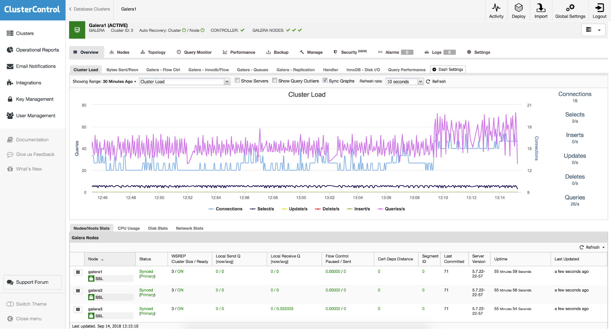
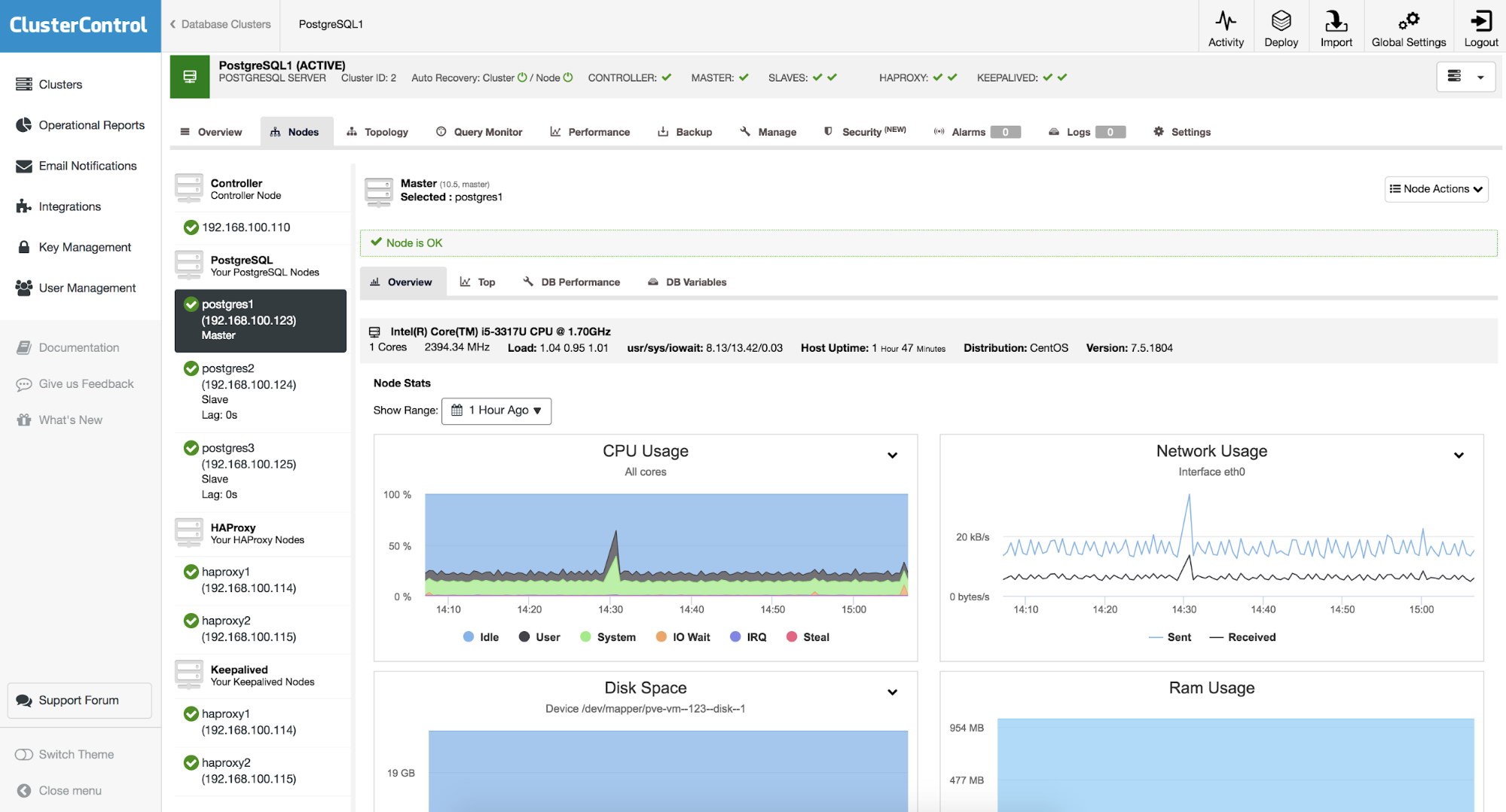
In the “Node” section, we can check the status and some metrics of our current servers in the cluster.

ClusterControl PostgreSQL Nodes
Download the Whitepaper Today
 
PostgreSQL Management & Automation with ClusterControl
Learn about what you need to know to deploy, monitor, manage and scale PostgreSQL

ClusterControl Failover

If the “Autorecovery” option is ON, in case of master failure, ClusterControl will promote the most advanced slave (if it is not in blacklist) to master as well as notify us of the problem. It also fails over the rest of the slaves to replicate from the new master.

HAProxy is configured with two different ports, one read-write and one read-only.

In our read-write port, we have our master server as online and the rest of our nodes as offline, and in the read-only port we have both the master and the slaves online.

When HAProxy detects that one of our nodes, either master or slave, is not accessible, it automatically marks it as offline and does not take it into account for sending traffic to it. Detection is done by healthcheck scripts that are configured by ClusterControl at time of deployment. These check whether the instances are up, whether they are undergoing recovery, or are read-only.

When ClusterControl promotes a slave to master, our HAProxy marks the old master as offline (for both ports) and puts the promoted node online (in the read-write port).

If our active HAProxy, which is assigned a Virtual IP address to which our systems connect, fails, Keepalived migrates this IP to our passive HAProxy automatically. This means that our systems are then able to continue to function normally.

In this way, our systems continue to operate normally and without our intervention.

Considerations

If we manage to recover our old failed master, it will NOT be re-introduced automatically to the cluster. We need to do it manually. One reason for this is that, if our replica was delayed at the time of the failure, if we add the old master to the cluster, it would mean loss of information or inconsistency of data across nodes. We might also want to analyze the issue in detail. If we just re-introduced the failed node into the cluster, we would possibly lose diagnostic information.

Also, if failover fails, no further attempts are made. Manual intervention is required to analyze the problem and perform the corresponding actions. This is to avoid the situation where ClusterControl, as the high availability manager, tries to promote the next slave and the next one. There might be a problem and we need to check this.

Security

One important thing we cannot forget before going into prod with our HA environment is to ensure the security of it.

There are several security aspects such as encryption, role management and access restriction by IP address. These topics were seen in depth in a previous blog, so we will only point them out in this blog.

In our PostgreSQL database, we have the pg_hba.conf file which handles the client authentication. We can limit the type of connection, the source IP or network, which database we can connect to and with which users. Therefore, this file is a very important piece for our security.

We can configure our PostgreSQL database from the postgresql.conf file, so it only listens on a specific network interface, and on a different port that the default port (5432), thus avoiding basic connection attempts from unwanted sources.

A correct user management, either using secure passwords or limiting access and privileges, is also an important piece of the security settings. It is recommended to assign the minimum amount of privileges possible to users, as well as to specify, if possible, the source of the connection.

We can also enable data encryption, either in transit or at rest, avoiding access to information to unauthorized persons.

The audit is important to know what happens or happened in our database. PostgreSQL allows you to configure several parameters for logging or even use the pgAudit extension for this task.

Last but not least, it is recommended to keep our database and servers up to date with the latest patches, to avoid security risks. For this ClusterControl gives us the possibility to generate operational reports to verify if we have update availables, and even help us to update our database.

Conclusion

In this blog we have reviewed some concepts regarding HA. We went through some possible architectures and the necessary components to set them effectively.

After that we explained how ClusterControl makes use of these components to deploy a complete HA environment for PostgreSQL.

And finally we reviewed some important security aspects to take into account before going live.

Bruce Momjian: Postgres 11 Features Presentation

Regina Obe: PostGIS 2.5.0rc2

$
0
0

The PostGIS development team is pleased to release PostGIS 2.5.0rc2.

Although this release will work for PostgreSQL 9.4 and above, to take full advantage of what PostGIS 2.5 offers, you should be running PostgreSQL 11beta3+ and GEOS 3.7.0 which were released recently.

Best served with PostgreSQL 11beta3.

2.5.0rc2

Changes since PostGIS 2.5.0rc1 release are as follows:

  • 4162, ST_DWithin documentation examples for storing geometry and radius in table (Darafei Praliaskouski, github user Boscop).
  • 4163, MVT: Fix resource leak when the first geometry is NULL (Raúl Marín)
  • 4172, Fix memory leak in lwgeom_offsetcurve (Raúl Marín)
  • 4164, Parse error on incorrectly nested GeoJSON input (Paul Ramsey)
  • 4176, ST_Intersects supports GEOMETRYCOLLECTION (Darafei Praliaskouski)
  • 4177, Postgres 12 disallows variable length arrays in C (Laurenz Albe)
  • 4160, Use qualified names in topology extension install (Raúl Marín)
  • 4180, installed liblwgeom includes sometimes getting used instead of source ones (Regina Obe)

View all closed tickets for 2.5.0.

After installing the binaries or after running pg_upgrade, make sure to do:

ALTER EXTENSION postgis UPDATE;

— if you use the other extensions packaged with postgis — make sure to upgrade those as well

ALTER EXTENSION postgis_sfcgal UPDATE;
ALTER EXTENSION postgis_topology UPDATE;
ALTER EXTENSION postgis_tiger_geocoder UPDATE;

If you use legacy.sql or legacy_minimal.sql, make sure to rerun the version packaged with these releases.


Jonathan Katz: Why Covering Indexes Are Incredibly Helpful

$
0
0

The PostgreSQL 11 release is nearly here (maybe in the next couple of weeks?!), and while a lot of the focus will be on the improvements to the overall performance of the system (and rightly so!), it's important to notice some features that when used appropriately, will provide noticeable performance improvements to your applications.

One example of such feature is the introduction of "covering indexes" for B-tree indexes. A covering index allows a user to perform an index-only scan if the looks in the query match the columns that are included in the index. You can specify the additional columns for the index using the "INCLUDE" keyword, e.g.

CREATE INDEX a_b_idx ONx(a,b)INLCUDE(c);

Theoretically, this can reduce the amount of I/O your query needs to use in order to retrieve information (traditionally, I/O is the biggest bottleneck on database systems). Additionally, the data types including in a covering index do not need to be B-tree indexable; you can add any data type to the INCLUDE part of a CREATE INDEX statement.

However, you still need to be careful for how you deploy covering indexes: each column you add to the index still takes up space on disk, and there is still a cost for maintaining the index, for examples, on row updates.

Understanding these trade offs, you can still apply covering indexes in very helpful ways that can significantly help your applications.

A Simple Example: Tracking Coffee Shop Visits

brian davis: Cost of a Join - Part 2: Enums, Wider Tables

$
0
0

A follow-up to the previous post where the performance of queries with many joins is investigated.

Great discussion on hacker news and r/programming brought up a couple ideas I hadn't considered.

  1. What about enums?
  2. What about tables with more columns?

I also figured it would be neat if other people could run these benchmarks with their own parameters / hardware.

So I adjusted my script to support enums and wider tables, and packaged it up into a tool anyone can use. It supports three different join types: enum, foreign keys, and what I'm calling "chained". The benchmark definitions are described in a json file which looks like this:

$ cat input.json
[
    {
        "join-type": "chained",
        "max-tables": 10,  # Queries will start by joining 2 tables, increasing by one until all tables are joined.  Number of tables joined will be the X axis on the plot.
        "max-rows": 10000,  # Benchmarks will be performed at 10 rows, 100 rows, etc. until max-rows is reached, creating a separate line on the plot for each.
        "extra_columns": 2,
        "max_id": 5,
        "create-indexes": true,
        "output-filename": "benchmark_1",
        "plot-title": "My Chained Benchmark Title"
    },
    {
        "join-type": "enums",
        "max-rows": 10000,  # Benchmarks will be performed at 10 rows in the primary table, increasing by a factor of 10 until max-rows is reached
        "max-enums": 100,  # Queries will start by selecting (and optionally filtering by) 1 enum column, increasing by one until max-enums is reached
        "possible-enum-values": 10,
        "extra-columns": 2,
        "where-clause": true,
        "output-filename": "benchmark_1",
        "plot-title": "My Enum Benchmark Title"
    },
    {
        "join-type": "foreign-keys",
        "max-primary-table-rows": 10000,  # Benchmarks will be performed at 10 rows in the primary table, increasing by a factor of 10 until max-rows is reached
        "max-fk-tables": 100,  # Queries will start by selecting from (and optionally filtering by) 1 foreign key table, increasing by one until max-fk-tables is reached
        "fk-rows": 100,
        "fk-extra-columns": 2,
        "extra-columns": 2,
        "where-clause": true,
        "output-filename": "benchmark_1",
        "plot-title": "My Foreign Key Benchmark Title"
    }
]

You supply it as input like so...

$ make build
$ PGHOST="localhost"PGDATABASE="join_test"PGUSER="brian"PGPASSWORD="pass" ./run_with_docker.sh input.json

It produces html charts as output, along with CSVs of the benchmark data.

results/chained_benchmark_1.html
results/chained_benchmark_1_10000_rows.csv
results/chained_benchmark_1_1000_rows.csv
results/chained_benchmark_1_100_rows.csv
results/chained_benchmark_1_10_rows.csv
results/enum_benchmark_1.html
results/enum_benchmark_1_10000_rows.csv
results/enum_benchmark_1_1000_rows.csv
results/enum_benchmark_1_100_rows.csv
results/enum_benchmark_1_10_rows.csv
results/foreign_key_benchmark_1.html
results/foreign_key_benchmark_1_10000_rows.csv
results/foreign_key_benchmark_1_1000_rows.csv
results/foreign_key_benchmark_1_100_rows.csv
results/foreign_key_benchmark_1_10_rows.csv

And that's it. You can specify as many benchmarks as you like in the json file, point it at a PostgreSQL instance and let it rip. I went ahead and did that with an RDS db.m4.large instance. Let's take a look at some results.


Enums vs Foreign Keys

The previous post looked at queries that joined one table to another, which was joined to another, which was joined to another, and so on. This is something we can't really do with enums, since an enum can't reference another enum. But we can change it up a bit and model something using foreign keys that is similar to what you might use an enum for. We can have one primary table with many integer columns, each referencing a different table that contains a number of text labels, and compare the performance of that to enums.

Foreign Keys

For the foreign key version, we'll create a primary table with 100 columns that each references a different table, each referenced table having 10 possible values, and we'll issue queries that select a value from one reference table, then two, then three, up to all 100, and we'll do this with the primary table containing 10, 100, 1,000, 10,000, and finally 100,000 rows.

Our primary table looks like this...

join_test=>\dprimary_tableTable"public.primary_table"Column|Type|Collation|Nullable|Default--------------+---------+-----------+----------+-------------------------------------------id|integer||notnull|nextval('primary_table_id_seq'::regclass)table_1_id|integer|||table_2_id|integer|||table_3_id|integer|||...table_100_id|integer|||Indexes:"primary_table_pkey"PRIMARYKEY,btree(id)Foreign-keyconstraints:"primary_table_table_1_id_fkey"FOREIGNKEY(table_1_id)REFERENCEStable_1(id)"primary_table_table_2_id_fkey"FOREIGNKEY(table_2_id)REFERENCEStable_2(id)"primary_table_table_3_id_fkey"FOREIGNKEY(table_3_id)REFERENCEStable_3(id)..."primary_table_table_100_id_fkey"FOREIGNKEY(table_100_id)REFERENCEStable_100(id)join_test=>

Our reference tables look like this...

join_test=>\dtable_5Table"public.table_5"Column|Type|Collation|Nullable|Default--------+---------+-----------+----------+-------------------------------------id|integer||notnull|nextval('table_5_id_seq'::regclass)label|text||notnull|Indexes:"table_5_pkey"PRIMARYKEY,btree(id)Referencedby:TABLE"primary_table"CONSTRAINT"primary_table_table_5_id_fkey"FOREIGNKEY(table_5_id)REFERENCEStable_5(id)join_test=>

And our queries look like this...

SELECTp.id,t1.labelASt1_label,t2.labelASt2_label,t3.labelASt3_label,...t5.labelASt5_labelFROMprimary_tableASpINNERJOINtable_1ASt1ONt1.id=p.table_1_idINNERJOINtable_2ASt2ONt2.id=p.table_2_idINNERJOINtable_3ASt3ONt3.id=p.table_3_idINNERJOIN...table_100ASt100ONt100.id=p.table_100_id;

Here are the results:

If we look at a table with 100,000 rows joining to fetch 5 of its associated labels, we're looking at 0.1s. If we're joining to fetch all 100 associated label values, and we only have 1,000 rows, we're still in that same ballpark of 0.17s. However, if we're fetching all 100 associated label values for 100,000 rows, we're now over 6 seconds.

It's worth noting that there's no where clause though, so this is, perhaps, not a super common use case in say, a web application. Still, it gives us something to compare enum performance to.

Enums

To replicate the above functionality with enums, we'll create a single table with 100 enum columns on it, each enum having 10 possible values, and we'll query one of those values, then two, then three, up to all 100, and we'll do this with the table containing 10, 100, 1,000, 10,000, and finally 100,000 rows.

Our enum using table looks like this...

join_test=>\dprimary_tableTable"public.primary_table"Column|Type|Collation|Nullable|Default-----------+-----------+-----------+----------+-------------------------------------------id|integer||notnull|nextval('primary_table_id_seq'::regclass)label_1|enum_1|||label_2|enum_2|||label_3|enum_3|||...label_100|enum_100|||Indexes:"primary_table_pkey"PRIMARYKEY,btree(id)join_test=>

And our queries look like this...

SELECTid,label_1,label_2,label_3,...label_100FROMprimary_table;

Wow! Enums really are faster. I didn't expect that to be the case, especially after reading that they are apparently implemented with a system table behind the scenes. Can't say I'm going to run out and replace all my reference tables with enums tomorrow, since there are some drawbacks. Existing values cannot be removed from an enum, and adding a new value cannot be executed inside a transaction block. But still. Interesting!

Filtering on Foreign Keys and Enums

With the ability to create tables like these already setup, I thought it might be interesting to see what happens if we filter on these values. So, same setup, but our queries will now have a where clause.

Foreign Key version:

SELECTp.id,t1.labelASt1_label,t2.labelASt2_label,t3.labelASt3_label,...t5.labelASt5_labelFROMprimary_tableASpINNERJOINtable_1ASt1ONt1.id=p.table_1_idINNERJOINtable_2ASt2ONt2.id=p.table_2_idINNERJOINtable_3ASt3ONt3.id=p.table_3_idINNERJOIN...table_100ASt100ONt100.id=p.table_100_idWHEREt1.label='My Label #1'ANDt2.label='My Label #1'ANDt3.label='My Label #1'AND...t100.label='My Label #1';

Foreign Key results:

Performance improves and the number of rows in the primary table doesn't seem to matter much. Here's the enum version with a where clause:

SELECTid,label_1,label_2,label_3,...label_100FROMprimary_tableWHERElabel_1='My Label #1'ANDlabel_2='My Label #1'ANDlabel_3='My Label #1'AND...label_100='My Label #1';

And the enum results:

Pretty great performance from enums. Whatever shortcuts PostgreSQL is able to take when filtering on these values, they certainly do have an impact. Filtering on all 100 enum columns for 100,000 rows takes only 0.06s.


Wider Tables

Wider tables are something we can test with the type of queries done in the prior post, the "chained" kind, where one table joins to another, which joins to another, etc. These wider tables will look like this, where we've added a number of columns between id and the reference to the previous table...

join_test=>\dtable_5Table"public.table_5"Column|Type|Collation|Nullable|Default-----------------+-----------------------+-----------+----------+-------------------------------------------id|integer||notnull|nextval('table_5_id_seq'::regclass)extra_column_1|charactervarying(20)|||'12345678901234567890'::charactervaryingextra_column_2|charactervarying(20)|||'12345678901234567890'::charactervaryingextra_column_3|charactervarying(20)|||'12345678901234567890'::charactervaryingextra_column_4|charactervarying(20)|||'12345678901234567890'::charactervaryingextra_column_5|charactervarying(20)|||'12345678901234567890'::charactervaryingextra_column_6|charactervarying(20)|||'12345678901234567890'::charactervaryingextra_column_7|charactervarying(20)|||'12345678901234567890'::charactervaryingextra_column_8|charactervarying(20)|||'12345678901234567890'::charactervaryingextra_column_9|charactervarying(20)|||'12345678901234567890'::charactervaryingextra_column_10|charactervarying(20)|||'12345678901234567890'::charactervaryingtable_4_id|integer|||Indexes:"table_5_pkey"PRIMARYKEY,btree(id)"table_5_table_4_id_idx"btree(table_4_id)Foreign-keyconstraints:"table_5_table_4_id_fkey"FOREIGNKEY(table_4_id)REFERENCEStable_4(id)Referencedby:TABLE"table_6"CONSTRAINT"table_6_table_5_id_fkey"FOREIGNKEY(table_5_id)REFERENCEStable_5(id)join_test=>

The benchmark script is sure to fill each one with real data

join_test=>select*fromtable_5limit1;-[RECORD1]---+---------------------id|1extra_column_1|12345678901234567890extra_column_2|12345678901234567890extra_column_3|12345678901234567890extra_column_4|12345678901234567890extra_column_5|12345678901234567890extra_column_6|12345678901234567890extra_column_7|12345678901234567890extra_column_8|12345678901234567890extra_column_9|12345678901234567890extra_column_10|12345678901234567890table_4_id|738Time:1.197msjoin_test=>

Our queries look like this...

SELECTcount(*)FROMtable_1ASt1INNERJOINtable_2ASt2ONt1.id=t2.table_1_idINNERJOINtable_3ASt3ONt2.id=t3.table_2_idINNERJOINtable_4ASt4ONt3.id=t4.table_3_idINNERJOIN...table_100ASt100ONt99.id=t100.table_99_idWHEREt1.id<=5;

Results using tables with 10 extra columns...

And results using tables with 100 extra columns...

Interesting that it matters, but also that it doesn't seem to matter much.

Conclusion

My takeaway from this is that enums really are faster in some cases, and that wider tables don't necessarily mean deal breaking slowdowns.

Another takeaway is that there are an infinite number of conditions and scenarios you might want to test. A few of them are even supported in the benchmarking tool if you'd like to try these cases for yourself:

  • Enums vs Foreign Keys with extra columns added to the primary table
  • Foreign Key benchmark with extra columns added to the referenced tables
  • Increasing the number of possible values in the enums / referenced tables

And of course, the number of rows / tables can be increased in general if you have the patience.

If you try any of that, let me know how it goes!

Sebastian Insausti: Custom Graphs to Monitor your MySQL, MariaDB, MongoDB and PostgreSQL Systems - ClusterControl Tips & Tricks

$
0
0

Graphs are important, as they are your window onto your monitored systems. ClusterControl comes with a predefined set of graphs for you to analyze, these are built on top of the metric sampling done by the controller. Those are designed to give you, at first glance, as much information as possible about the state of your database cluster. You might have your own set of metrics you’d like to monitor though. Therefore ClusterControl allows you to customize the graphs available in the cluster overview section and in the Nodes -> DB Performance tab. Multiple metrics can be overlaid on the same graph.

Cluster Overview tab

Let’s take a look at the cluster overview - it shows the most important information aggregated under different tabs.

Cluster Overview Graphs

You can see graphs like “Cluster Load” and “Galera - Flow Ctrl” along with couple of others. If this is not enough for you, you can click on “Dash Settings” and then pick “Create Board” option. From there, you can also manage existing graphs - you can edit a graph by double-clicking on it, you can also delete it from the tab list.

Dashboard Settings
Dashboard Settings

When you decide to create a new graph, you’ll be presented with an option to pick metrics that you’d like to monitor. Let’s assume we are interested in monitoring temporary objects - tables, files and tables on disk. We just need to pick all three metrics we want to follow and add them to our new graph.

New Board 1
New Board 1

Next, pick some name for our new graph and pick a scale. Most of the time you want scale to be linear but in some rare cases, like when you mix metrics containing large and small values, you may want to use logarithmic scale instead.

New Board 2
New Board 2

Finally, you can pick if your template should be presented as a default graph. If you tick this option, this is the graph you will see by default when you enter the “Overview” tab.

Once we save the new graph, you can enjoy the result:

New Board 3
New Board 3

Node Overview tab

In addition to the graphs on our cluster, we can also use this functionality on each of our nodes independently. On the cluster, if we go to the “Nodes” section and select some of them, we can see an overview of it, with metrics of the operating system:

Node Overview Graphs

As we can see, we have eight graphs with information about CPU usage, Network usage, Disk space, RAM usage, Disk utilization, Disk IOPS, Swap space and Network errors, which we can use as a starting point for troubleshooting on our nodes.

ClusterControl
Single Console for Your Entire Database Infrastructure
Find out what else is new in ClusterControl

DB Performance tab

When you take a look at the node and then follow into DB Performance tab, you’ll be presented with a default of eight different metrics. You can change them or add new ones. To do that, you need to use “Choose Graph” button:

DB Performance Graphs

You’ll be presented with a new window, that allows you to configure the layout and the metrics graphed.

DB Performance Graphs Settings

Here you can pick the layout - two or three columns of graphs and number of graphs - up to 20. Then, you may want to modify which metrics you’d want to see plotted - use drop-down dialog boxes to pick whatever metric you’d like to add. Once you are ready, save the graphs and enjoy your new metrics.

We can also use the Operational Reports feature of ClusterControl, where we will obtain the graphs and the report of our cluster and nodes in a HTML report, that can be accessed through the ClusterControl UI, or schedule it to be sent by email periodically.

These graphs help us to have a complete picture of the state and behavior of our databases.

Laurenz Albe: Correlation of PostgreSQL columns explained

$
0
0

Better correlation helps in real life too

After you ANALYZE a PostgreSQL table to collect value distribution statistics, you will find the gathered statistics for each column in the pg_stats system view. This article will explain the meaning of the correlation column and its impact on index scans.

Physical vs. logical ordering

Most common PostgreSQL data types have an ordering: they support the operators <, <=, =, >= and >.
Such data types can be used with a B-tree index (the “standard” index type).

The values in a column of such a type provide a logical ordering of the table rows. An index on this column will be sorted according to that ordering.

A PostgreSQL table consists of one or more files of 8KB blocks. The order in which the rows are stored in the file is the physical ordering.
You can examine the physical ordering of the rows by selecting the ctid system column: it contains the block number and the item number inside the block, which describe the physical location of the table row.

Correlation

The correlation for a column is a value between -1 and 1. It tells how good the match between logical and physical ordering is.

  • If the correlation is 1, the rows are stored in the table file in ascending column order; if it is -1, they are stored in descending order.
  • Values between -1 and 1 mean a less perfect match.
  • A value of 0 means that there is no connection between the physical and the logical order.

Why should I care?

You will create indexes on your tables for faster access (but not too many!).
The correlation of a column has an impact on the performance of an index scan.

During an index scan, the whole index or part of it are read in index sequential order. For each entry that is found, the corresponding row is fetched from the table (this is skipped in an “index only scan”, but that is a different story).

If the correlation of the indexed column is close to zero, the fetched rows will be from all over the table. This will result in many randomly distributed reads of many different table blocks.

However, if the correlation is close to 1 or -1, the next row fetched during the index scan tends to be in the same or the next table block as the previous row.

High correlation has two advantages:

  1. Blocks read by the database are cached in shared memory. Consequently, if many of the table rows fetched during the index scan are located in the same table block, only few blocks have to be read from storage.
  2. The blocks that have to be read from storage are next to each other. This leads to sequential I/O, which on spinning disks is substantially faster than random I/O.

An example

Let’s create two tables with identical content, but different correlation:

CREATE TABLE corr (id, val) AS
   SELECT i, 'some text ' || i
   FROM generate_series(1, 100000) AS i;

CREATE INDEX corr_idx ON corr (id);

VACUUM (ANALYZE) corr;

SELECT correlation FROM pg_stats
WHERE tablename = 'corr' AND attname = 'id';

 correlation 
-------------
           1
(1 row)

CREATE TABLE uncorr AS
   SELECT * FROM corr
   ORDER BY random();

CREATE INDEX uncorr_idx ON uncorr (id);

VACUUM (ANALYZE) uncorr;

SELECT correlation FROM pg_stats
WHERE tablename = 'uncorr' AND attname = 'id';

 correlation 
-------------
 -0.00522369
(1 row)

We disable bitmap index scans so that we can compare index scans on both tables.
Then we check how index scans perform:

SET enable_bitmapscan = off;

EXPLAIN (ANALYZE, BUFFERS)
SELECT * FROM corr WHERE id BETWEEN 1001 AND 1300;

                    QUERY PLAN
---------------------------------------------------
 Index Scan using corr_idx on corr
       (cost=0.29..15.23 rows=297 width=19)
       (actual time=0.108..0.732 rows=300 loops=1)
   Index Cond: ((id >= 1001) AND (id <= 1300))
   Buffers: shared hit=6
 Planning time: 0.456 ms
 Execution time: 1.049 ms
(5 rows)

EXPLAIN (ANALYZE, BUFFERS)
SELECT * FROM uncorr WHERE id BETWEEN 1001 AND 1300;

                    QUERY PLAN
---------------------------------------------------
 Index Scan using uncorr_idx on uncorr
       (cost=0.29..978.15 rows=298 width=19)
       (actual time=0.105..2.352 rows=300 loops=1)
   Index Cond: ((id >= 1001) AND (id <= 1300))
   Buffers: shared hit=303
 Planning time: 0.548 ms
 Execution time: 2.736 ms
(5 rows)

Now 2.7 milliseconds is not so bad, but that is only because all blocks were already in shared buffers.
If a part of these blocks has to be read from disk, the 303 blocks from the second query will do much worse than the 6 from the first!

In the second query, each result row was found in a different table block. This caused 300 blocks to be touched. The remaining three blocks are index blocks.

The first query touches only three table blocks:

SELECT ctid, id FROM corr
WHERE id BETWEEN 1001 AND 1300;

  ctid   |  id  
---------+------
 (6,58)  | 1001
 (6,59)  | 1002
 (6,60)  | 1003
 (6,61)  | 1004
 (6,62)  | 1005
 (6,63)  | 1006
 (6,64)  | 1007
 ...
 (8,37)  | 1294
 (8,38)  | 1295
 (8,39)  | 1296
 (8,40)  | 1297
 (8,41)  | 1298
 (8,42)  | 1299
 (8,43)  | 1300
(300 rows)

Indeed, all rows are contained in the table blocks 6, 7 and 8!

Correlation and the optimizer

The PostgreSQL optimizer estimates the cost of the possible ways to execute an SQL statement.

With the use of the correlation it can give better estimates of the cost of an index scan, leading to better plan choices.

The PostgreSQL optimizer will prefer index scans if the correlation is close to 1 or -1.

Correlation and BRIN indexes

PostgreSQL 9.5 introduced the BRIN index (block range index).

This index works be storing the minimum and maximum of all values for ranges of table blocks. It is only useful for columns with perfect correlation. Its advantage over the B-tree index is its much smaller size, which makes it an interesting option for large tables.

How to make use of correlation?

If you need to efficiently scan bigger portions of an index, it is good to keep the table in index order.

There are no “index ordered tables” in PostgreSQL.
Still, high correlation for a column can be maintained in two ways:

  1. Automatically:

    If the table rows are inserted in logical column order and there are no updates or deletes on the table, the physical ordering will be identical to the logical ordering. Good examples for that are primary key columns generated by sequences or measurements with a timestamp.

    Since correlation is always perfect in this case, a BRIN index can be an interesting option.

    If you want to remove old data from a table without disrupting the physical ordering, you can use table partitioning.

  2. Clustering:

    The SQL statement CLUSTER can be used to rewrite a table so that the physical ordering is identical to the logical ordering of an index.

    However, subsequent modifications of the table will reduce the correlation again. Because of that, you need to re-cluster the table regularly to maintain high correlation. This is annoying, because CLUSTER blocks all concurrent access to the table.

The post Correlation of PostgreSQL columns explained appeared first on Cybertec.

Craig Kerstiens: Use cases for followers (read replicas) in Postgres

$
0
0

Citus extends Postgres to be a horizontally scalable database. By horizontally scalable, we mean the data is spread across multiple machines, and you’re able to scale not only storage but also memory and compute—thus providing better performance. Without using something like Citus to transform PostgreSQL into a distributed database, sure you can add read replicas to scale, but you’re still maintaining a single copy of your data. When you run into scaling issues with your Postgres database, adding a read replica and offloading some of your traffic to your read replica is a common bandaid to slow down the bleeding, but it is only a matter of time until even that doesn’t work any further. Whereas with Citus, scaling out your database is as simple as dragging a slider and rebalancing your data.

Are read replicas still useful with horizontally scalable databases?

But that leaves a question, are read-replicas still useful? Well, sure they are.

In Citus Cloud (our fully-managed database as a service), we have support for read replicas, in our case known as followers. Follower clusters leverage much of our same underlying disaster recovery infrastructure that forks leverage, but support a very different set of use cases.

Previously we talked about how forks can be used in Citus Cloud to get a production set of data over to staging that can help with testing migrations, rebalancing, or SQL query optimization. Forks are often used as a one-off for a short period of time. In contrast, followers are often long running Citus database clusters that can be a key mechanism to run your business, helping you get insights when you need them.

Follower cluster is often only a few seconds (if any) behind your primary database cluster

A follower cluster receives all updates from the primary Citus cluster in an asynchronous fashion. Often followers are only a few seconds (if any) behind your primary database cluster, though can lag at times by a few minutes. Followers have a full copy of your data, but reside on a separate cluster. This means you have a separate copy of the data with its own compute power, memory, and disk.

Fun fact about follower formations, you can create them cross-region as well. Want to have a full copy of your database in another region that you can fail over to in a disaster situation? Want to provide lower latency on particular reads for a different geography? A cross-region Citus follower can help.

Followers = useful to separate analytics workloads from core production activity

So when are followers useful in Citus? Followers are most helpful for analytical workloads that may be longer running. Want to compute some complex report against your entire data set? Performing ETL from your primary database into some other data warehouse where data is cleansed and obfuscated before it goes in?

Each of these use cases may be important for your business, but long-running SQL queries compete for the same resources as your primary workload for the database. This competition for performance can result in performance issues at times for the primary workload in your database. By splitting this analytical workload out to operate on a Citus follower cluster, you can give your internal data analysts the access they need, without having to subject them to the same code review processes of production—all while keeping your production database safe.

Read replicas and followers still have a place

While using read replicas as an attempt to scale your main application may introduce all sorts of unnecessary complexity and create more work than problems that are solved, read replicas do still have their place. When using the Citus extension to Postgres to solve the problem of scaling performance, you can create follower formations (aka read replicas) to provide access to your data internally without having to risk production availability. It’s a powerful combination.

Viewing all 9681 articles
Browse latest View live


<script src="https://jsc.adskeeper.com/r/s/rssing.com.1596347.js" async> </script>