Declarative partitioning got some attention in the PostgreSQL 12 release, with some very handy features. There has been some pretty dramatic improvement in partition selection (especially when selecting from a few partitions out of a large set), referential integrity improvements, and introspection. In this article, we’re going to tackle the referential integrity improvement first. This […]
↧
Kirk Roybal: Partitioning enhancements in PostgreSQL 12
↧
Jobin Augustine: BRIN Index for PostgreSQL: Don’t Forget the Benefits

 BRIN Index was introduced in PostgreSQL 9.5, but many users postponed the usage of it in their design and development just because it was “new”. But now we understand that it has stood the test-of-time! It is time to reconsider BRIN if you have not done it yet. I often see users who forget there is a provision to select the type of Index by specifying USING clause when creating an index.
BRIN Index is a revolutionary idea in indexing first proposed by PostgreSQL contributor Alvaro Herrera. BRIN stands for “Block Range INdex”. A block range is a group of pages adjacent to each other, where summary information about all those pages is stored in Index. For example, Datatypes like integers – dates where sort order is linear – can be stored as min and max value in the range. Other database systems including Oracle announced similar features later. BRIN index often gives similar gains as Partitioning a table.
BRIN usage will return all the tuples in all the pages in the particular range. So the index is lossy and extra work is needed to further filter out records. So while one might say that is not good, there are a few advantages.
- Since only summary information about a range of pages is stored, BRIN indexes are usually very small compared to B-Tree indexes. So if we want to squeeze the working set of data to shared_buffer, this is a great help.
- Lossiness of BRIN can be controlled by specifying pages per range (discussed in a later section)
- Offloads the summarization work to vacuum or autovacuum. So the overhead of index maintenance on transaction / DML operation is minimal.
Putting BRIN into a test
Let’s take a simple example to examine the benefits of BRIN index by creating a simple table.
postgres=# CREATE TABLE testtab (id int NOT NULL PRIMARY KEY,date TIMESTAMP NOT NULL, level INTEGER, msg TEXT);
CREATE TABLE
Now let’s Insert some data into this table.
postgres=# INSERT INTO testtab (id, date, level, msg) SELECT g, CURRENT_TIMESTAMP + ( g || 'minute' ) :: interval, random() * 6, md5(g::text) FROM generate_series(1,8000000) as g;
INSERT 0 8000000
Please note that values in id column and date columns keep increasing for new records, which is common for transaction records. This is an important property which BRIN make use off.
A query at this stage may have to do a full scan of the table and it will be quite expensive.
postgres=# explain analyze select * from public.testtab where date between '2019-08-08 14:40:47.974791' and '2019-08-08 14:50:47.974791';
                                                                          QUERY PLAN
---------------------------------------------------------------------------------------------------------------------------------------------------------------
Gather  (cost=1000.00..133476.10 rows=11 width=49) (actual time=31.835..1766.409 rows=11 loops=1)
  Workers Planned: 2
  Workers Launched: 2
  -> Parallel Seq Scan on testtab  (cost=0.00..132475.00 rows=5 width=49) (actual time=1162.029..1739.713 rows=4 loops=3)
        Filter: ((date >= '2019-08-08 14:40:47.974791'::timestamp without time zone) AND (date <= '2019-08-08 14:50:47.974791'::timestamp without time zone))
        Rows Removed by Filter: 2666663
Planning Time: 0.296 ms
Execution Time: 1766.454 ms
(8 rows)
As we can see above, PostgreSQL employs 2 workers and does the scan in parallel, where it takes 1766.454 ms. In a nutshell, it is heavy on the system and takes a good amount of time.
As usual, our tendency is to create an index on the filtering column. (B-Tree by default)
postgres=# create index testtab_date_idx  on testtab(date);
CREATE INDEX
Now let’s see how the previous SELECT query works:
postgres=# explain analyze select * from public.testtab where date between '2019-08-08 14:40:47.974791' and '2019-08-08 14:50:47.974791';
                                                                        QUERY PLAN
-------------------------------------------------------------------------------------------------------------------------------------------------------------
Index Scan using testtab_date_idx on testtab  (cost=0.43..8.65 rows=11 width=49) (actual time=1.088..1.090 rows=11 loops=1)
  Index Cond: ((date >= '2019-08-08 14:40:47.974791'::timestamp without time zone) AND (date <= '2019-08-08 14:50:47.974791'::timestamp without time zone))
Planning Time: 22.225 ms
Execution Time: 2.657 ms
(4 rows)
Obviously, B-Tree is lossless, and it can give a tremendous boost to the performance and efficiency of SELECT queries, especially when Index is freshly created. But a B-Tree index has following side effects:
- There will be a reasonable penalty for DMLs
- Index size can go big and consume a good amount of shared_buffers
- The random page seeks, especially when index pages are not cached, can become expensive.
It will be interesting to check the Index to table size ratio of this fresh index.
postgres=# \di+ testtab_date_idx;
List of relations
Schema | Name | Type | Owner | Table | Size | Description
--------+------------------+-------+----------+---------+--------+-------------
public | testtab_date_idx | index | postgres | testtab | 171 MB |
(1 row)
So we have B-Tree index 171MB for a 1.3GB table. So Index to table size ratio is 0.13, for this is a fresh index.
But this index-table ratio can keep deteriorating over time as index undergoes continuous updates. Index ratio crossing 0.5 is common in many production environments. As the ratio becomes bad, the efficiency of the index goes bad and it starts occupying more shared buffers.
Things get much worse if the table grows to a bigger size (hundreds of GB or TB) as Index also grows in the same ratio. The impact of B-Tree index on DMLs is heavy – sometimes I measured up to 30% overhead especially for bulk loads.
Now let’s see what happens if we replace a B-Tree index with a BRIN index.
postgres=# create index testtab_date_brin_idx  on testtab using brin (date);
CREATE INDEX
The very first observation is that the impact of Index on the same bulk insert operation is measured to be 3% which is within my noise/error limits. 30% overhead Vs 3% overhead.
If we consider the size of the newly created BRIN index:
postgres=# \di+ testtab_date_brin_idx;
                                List of relations
Schema |         Name          | Type  |  Owner   |  Table  | Size  | Description
--------+-----------------------+-------+----------+---------+-------+-------------
public | testtab_date_brin_idx | index | postgres | testtab | 64 kB |
(1 row)
As we can see it is just 64kB! 171MB of B-Tree index Vs 64 kb of BRIN index.
So far BRIN wins my heart. Now its time to look at how much query performance improvement it can bring in.
postgres=# explain analyze select * from public.testtab where date between '2019-08-08 14:40:47.974791' and '2019-08-08 14:50:47.974791';
                                                                            QUERY PLAN
-------------------------------------------------------------------------------------------------------------------------------------------------------------------
Bitmap Heap Scan on testtab  (cost=20.03..33406.84 rows=11 width=49) (actual time=62.762..87.471 rows=11 loops=1)
  Recheck Cond: ((date >= '2019-08-08 14:40:47.974791'::timestamp without time zone) AND (date <= '2019-08-08 14:50:47.974791'::timestamp without time zone))
  Rows Removed by Index Recheck: 12405
  Heap Blocks: lossy=128
  -> Bitmap Index Scan on testtab_date_brin_idx  (cost=0.00..20.03 rows=12403 width=0) (actual time=1.498..1.498 rows=1280 loops=1)
        Index Cond: ((date >= '2019-08-08 14:40:47.974791'::timestamp without time zone) AND (date <= '2019-08-08 14:50:47.974791'::timestamp without time zone))
Planning Time: 0.272 ms
Execution Time: 87.703 ms
(8 rows)
As I expected, it is not that efficient as a fully cached B-Tree index. However, performance improvement from 1766.454 ms to 87.703 ms means approximately 20 times better! That’s with a single worker consuming fewer resources. With just a 64kb Overhead, the cost-benefit of BRIN is very positive.
Storage and maintenance
As we saw the BRIN index uses much less space compared to normal B-Tree index, but the lossy index can reduce the effectiveness of Index. Luckily this can be adjusted using the storage parameter pages_per_range. BRIN stores entries for a range of pages in the corresponding table. The larger the range of pages, the smaller the index, and it gets lossier.
create index testtab_date_brin_idx on testtab using brin (date) with (pages_per_range = 32);
As we already discussed, part of the index maintenance during DML is offloaded to vacuum. In fact, there are 2 cases.
- Pages in the table which are already summarized are updated
- New pages which are not part of the summary.
In the first case, summary in BRIN is updated straight away along with DML. But if new pages are not summarized already, it will be done by VACUUM or AUTOVACUUM.
There are 2 functions provided for this. A high-level, function call which can be executed against the index like:
postgres=# select brin_summarize_new_values('testtab_date_brin_idx'::regclass);
brin_summarize_new_values
---------------------------
2577
(1 row)
This summarizes all ranges that are not currently summarized. The return value indicates the number of new page range summaries that were inserted into the index. This function operates on the top of a lower-level function brin_summarize_range which accepts the range of pages.
postgres=# SELECT brin_summarize_range('testtab_date_brin_idx', 10);
brin_summarize_range
----------------------
0
(1 row)
A key point to note is that auto-summarization is off by default, which we can enable by storage parameter auto summarize:
postgres=# alter index testtab_date_brin_idx set (pages_per_range = 64,autosummarize = on);
ALTER INDEX
In this case, automatic summarization will be executed by autovacuum as insertions occur.
Limitation:
BRIN indexes are efficient if the ordering of the key values follows the organization of blocks in the storage layer. In the simplest case, this could require the physical ordering of the table, which is often the creation order of the rows within it, to match the key’s order. Keys on generated sequence numbers or created data are best candidates for BRIN index. As a consequence, it is meaningful to have only one BRIN index on a table.
↧
↧
Kaarel Moppel: The mysterious “backend_flush_after” configuration setting
The above-mentioned PostgreSQL server configuration parameter was introduced already some time ago, in version 9.6, but has been flying under the radar so to say and had not caught my attention previously. Until I recently was pasted (not being on Twitter) a tweet from one of the Postgres core developers Andres Freund, that basically said– if your workload is bigger than Shared Buffers, you should enable the “ backend_flush_after” parameter for improved throughput and also jitter. Hmm, who wouldn’t like an extra boost on performance for free? FOMO kicked in… but before adding this parameter to my “standard setup toolbox” I hurried to test things out – own eye is king! So here a small test and my conclusion on effects of enabling (not enabled by default!) “backend_flush_after”.
What does this parameter actually do?
Trying to interpret the documentation (link here) in my own wording – “backend_flush_after” is basically designed to enable sending “hints” to the OS, that if user has written more than X bytes (configurable from 0 to max. 2MB) it would be very nice if the kernel could already do some flushing of recently changed data files in the background, so that when the “checkpointer” comes or the kernel’s “dirty” limit is reached, there would be less bulk “fsyncing” to do – meaning less IO contention (spikes) for our user sessions, thus smoother response times.
Be warned though – unlike most Postgres settings this one actually is not guaranteed to function, and currently only can work on Linux systems, having sync_file_range() functionality available – which again depends on kernel version and used file system. So in short this explains why the parameter has not gotten too much attention. Similar story actually also with the “sister” parameters – “bgwriter_flush_after”, “checkpoint_flush_after”, “wal_writer_flush_after”…with the difference that they are already enabled by default!
NB! Also note that this parameter, being controlled and initiated by Postgres, might be the only way to influence the kernel IO subsystem when using some managed / cloud PostgreSQL service!
Test setup
- Hardware: 4vCPU, 8GB, 160 GB local SSD, Ubuntu 18.04 (dirty_ratio=20, dirty_background_ratio=10, no Swap) droplet on DigitalOcean (Frankfurt)
- Software: PostgreSQL 11.4 at defaults, except – checkpoint_completion_target=0.9 (which is quite a typical setting to “smooth” IO), shared_buffers=’2GB’
- Test case: standard “pgbench” OLTP runs with 2 clients per CPU, 2h runs i.e.: “pgbench -T 7200 -c 8 -M prepared –random-seed=5432”
- Test 1 settings: Workload fitting into Shared Buffers (–scale=100)
- Test 2 settings: Workload 4x bigger than RAM (–scale=2200). FYI – to calculate the needed “scale factor” I use this calculator
As you might have noticed – although the tweet mentioned workloads bigger than Shared Buffers, in the spirit of good old “doubt everything”, I decided to test both cases still:)
Test results
With Test 1, where workload was fitting into shared_buffers, there’s actually nothing worthwhile to mention – my radars picked up no remotely significant difference, Andres was right! And basically test #2 also confirmed what was declared – but see the table below for numbers. NB! Numbers were measured on server side from “pg_stat_statements” and during the tests system CPU utilization was on average around ~55% and IO-wait (vmstat “wa” column) showing 25% which is much more than a typical system would exhibit but what should highlight the “backend_flush_after” IO optimizations better. Also note that the results table includes numbers only for the main UPDATE “pgbench_accounts” SQL statement as differences for the other mini-tables (which get fully cached) were on the “noise level”.
UPDATE pgbench_accounts SET abalance = abalance + $1 WHERE aid = $2
| Test | Mean time (ms) | Change (%) | Stddev time (ms) | Change (%) |
|---|---|---|---|---|
| Workload=4x mem., backend_flush_after=0 (default) | 0.637 | – | 0.758 | – |
| Workload=4x mem., backend_flush_after=512kB | 0.632 | -0.8 | 0.606 | -20.0 |
| Workload=4x mem., backend_flush_after=2MB | 0.609 | -4.4 | 0.552 | -27.2 |
Conclusion
First off – as it was a very simple test, I wouldn’t assign too much importance to the numbers themselves. But it showed that indeed, the “backend_flush_after” setting makes things a bit better when using the biggest “chunk size”, especially visible with transaction time standard deviations…and more importantly – it doesn’t also make things worse! So for heavily loaded setups I’ll use it without fear in the future, especially with spinning disks (if anyone still using them), where the difference should be even more pronounced. Bear in mind though that when it comes to Linux kernel disk subsystem, there’s a bunch of other parameters that are relevant, like “dirty_ratio”, “dirty_background_ratio”, “swappiness” and the type of scheduler, and the effects of tuning those could be even bigger!
The post The mysterious “backend_flush_after” configuration setting appeared first on Cybertec.
↧
Luca Ferrari: Suggesting Single-Column Primary Keys (almost) Automatically
Is it possible to infer primary keys automatically? If it, I’m not able at doing that, but at least I can try.
Suggesting Single-Column Primary Keys (almost) Automatically
A comment on my previous blog post about generating primary keys with a procedure made me think about how to inspect a table to understand which columns can be candidates for primary keys.
Of course, this does make sense (at least to me) for single-column constraints only, because multi column constraint require a deep knowledge about the data. Anyway, here it is my first attempt:
CREATEORREPLACEFUNCTIONf_suggest_primary_keys(schemaztextDEFAULT'public',tableztextDEFAULTNULL)RETURNSSETOFtextAS$CODE$DECLAREcurrent_statsrecord;is_uniqueboolean;is_primary_keyboolean;could_be_uniqueboolean;could_be_primary_keyboolean;current_constraintchar(1);current_alter_tabletext;BEGINRAISEDEBUG'Inspecting schema % (table %)',schemaz,tablez;FORcurrent_statsINSELECTs.*,n.oidASnspoid,c.oidASreloidFROMpg_statssJOINpg_classcONc.relname=s.tablenameJOINpg_namespacenONn.oid=c.relnamespaceWHEREs.schemaname=schemazANDc.relkind='r'ANDn ↧
Craig Kerstiens: Postgres tips for the average and power user
Personally I’m a big fan of email, just like blogging. To me a good email thread can be like a good novel where you’re following along always curious for what comes next. And no, I don’t mean the ones where there is an email to all-employees@company.com and someone replies all, to only receive reply-all’s to not reply-all. I mean ones like started last week internally among the Azure Postgres team.
The first email was titled: Random Citus development and psql tips, and from there it piled on to be more and more tips and power user suggestions for Postgres. Some of these tips are relevant if you’re working directly on the Citus codebase, others relevant as anyone that works with Postgres, and some useful for debugging Postgres internals. While the thread is still ongoing here is just a few of the great tips:
In psql, tag your queries and use Ctrl+R
Psql supports Ctrl+R to search previous queries you ran. For demos and when testing complex scenarios, I like adding a little comment to queries that then becomes the tag by which I can later find the query:
#SELECTcount(*)FROMtest;-- full count┌───────┐│count│├───────┤│0│└───────┘(1row)Time:127.124ms(reverse-i-search)`f': SELECT count(*) FROM test; -- full count
In most cases, 2-3 letters is going to be enough to find the query.
Better psql output
I find \x lacking, but pspg is great. It is available from PGDG via sudo yum install -y pspg or the equivalent on your system. I have the following .psqlrc which sets up pspg with a very minimalistic configuration:
$ cat > ~/.psqlrc
\timing on
\pset linestyle unicode
\pset border 2
\setenv PAGER 'pspg --no-mouse -bX --no-commandbar --no-topbar'\set HISTSIZE 100000
Get a stack trace for an error
In psql:
#SELECTpg_backend_pid();┌────────────────┐│pg_backend_pid│├────────────────┤│156796│└────────────────┘(1row)In another shell:
$ gdb -p 156796
(gdb) b errfinish
Breakpoint 1 at 0x83475b: file elog.c, line 251.
(gdb) c
Continuing.
Back in psql:
#SELECT1/0;Back in gdb:
Breakpoint 1, errfinish (dummy=0) at elog.c:414
414     {(gdb) bt
#0  errfinish (dummy=0) at elog.c:414#1  0x00000000007890f3 in int4div (fcinfo=<optimized out>) at int.c:818#2  0x00000000005f543c in ExecInterpExpr (state=0x1608000, econtext=0x1608900, isnull=0x7ffd27d1ad7f) at execExprInterp.c:678
...
Generating and inserting fake data
I know there are a lot of ways to generate fake data, but if you want something simple and quick you can do it directly in SQL:
CREATETABLEsome_table(idbigserialPRIMARYKEY,afloat);SELECTcreate_distributed_table('some_table','id');INSERTINTOsome_table(a)SELECTrandom()*100000FROMgenerate_series(1,1000000)i;-- 2 secs (40MB)INSERTINTOsome_table(a)SELECTrandom()*100000FROMgenerate_series(1,10000000)i;-- 20 secs (400MB)INSERTINTOsome_table(a)SELECTrandom()*100000FROMgenerate_series(1,100000000)i;-- 300 secs (4GB)INSERTINTOsome_table(a)SELECTrandom()*100000FROMgenerate_series(1,1000000000)i;-- 40 mins (40GB)A better pg_stat_activity
We’ve talked about pg_stat_statementsbefore, but less about pg_stat_activity. Pg_stat_activity will show you information about currently running queries. Though it’s default view gets improved with the following query, and is easy to tweak as well:
SELECTpid,-- procpid,-- usename, substring(query,0,100)asquery,query_start,-- backend_start,backend_type,stateFROMpg_stat_activity--WHERE-- state='active'ORDERBYquery_startASC;Managing multiple versions of Postgres
For many people one version of Postgres is enough, but if you’re working with different versions in production it can be useful to have them locally as well for dev/prod parity. pgenv is a tool that helps you manage and easily swap between Postgres versions.
What are your tips?
As our email thread goes on we may create another post on useful tips, but I’d also love to hear from you. Have some useful tips for working with Postgres, let us hear them and help share with others @citusdata.
Big thanks to Onder, Marco, Furkan on the team for contributing tips to the thread
↧
↧
Sebastian Insausti: Scaling Postgresql for Large Amounts of Data

Nowadays, it’s common to see a large amount of data in a company’s database, but depending on the size, it could be hard to manage and the performance could be affected during high traffic if we don’t configure or implement it in a correct way. In general, if we have a huge database and we want to have a low response time, we’ll want to scale it. PostgreSQL is not the exception to this point. There are many approaches available to scale PostgreSQL, but first, let’s learn what scaling is.
Scalability is the property of a system/database to handle a growing amount of demands by adding resources.
The reasons for this amount of demands could be temporal, for example, if we’re launching a discount on a sale, or permanent, for an increase of customers or employees. In any case, we should be able to add or remove resources to manage these changes on the demands or increase in traffic.
In this blog, we’ll look at how we can scale our PostgreSQL database and when we need to do it.
Horizontal Scaling vs Vertical Scaling
There are two main ways to scale our database...
- Horizontal Scaling (scale-out): It’s performed by adding more database nodes creating or increasing a database cluster.
- Vertical Scaling (scale-up): It’s performed by adding more hardware resources (CPU, Memory, Disk) to an existing database node.

For Horizontal Scaling, we can add more database nodes as slave nodes. It can help us to improve the read performance balancing the traffic between the nodes. In this case, we’ll need to add a load balancer to distribute traffic to the correct node depending on the policy and the node state.
To avoid a single point of failure adding only one load balancer, we should consider adding two or more load balancer nodes and using some tool like “Keepalived”, to ensure the availability.
As PostgreSQL doesn’t have native multi-master support, if we want to implement it to improve the write performance we’ll need to use an external tool for this task.
For Vertical Scaling, it could be needed to change some configuration parameter to allow PostgreSQL to use a new or better hardware resource. Let’s see some of these parameters from the PostgreSQL documentation.
- work_mem: Specifies the amount of memory to be used by internal sort operations and hash tables before writing to temporary disk files. Several running sessions could be doing such operations concurrently, so the total memory used could be many times the value of work_mem.
- maintenance_work_mem: Specifies the maximum amount of memory to be used by maintenance operations, such as VACUUM, CREATE INDEX, and ALTER TABLE ADD FOREIGN KEY. Larger settings might improve performance for vacuuming and for restoring database dumps.
- autovacuum_work_mem: Specifies the maximum amount of memory to be used by each autovacuum worker process.
- autovacuum_max_workers: Specifies the maximum number of autovacuum processes that may be running at any one time.
- max_worker_processes: Sets the maximum number of background processes that the system can support. Specify the limit of the process like vacuuming, checkpoints, and more maintenance jobs.
- max_parallel_workers: Sets the maximum number of workers that the system can support for parallel operations. Parallel workers are taken from the pool of worker processes established by the previous parameter.
- max_parallel_maintenance_workers: Sets the maximum number of parallel workers that can be started by a single utility command. Currently, the only parallel utility command that supports the use of parallel workers is CREATE INDEX, and only when building a B-tree index.
- effective_cache_size: Sets the planner's assumption about the effective size of the disk cache that is available to a single query. This is factored into estimates of the cost of using an index; a higher value makes it more likely index scans will be used, a lower value makes it more likely sequential scans will be used.
- shared_buffers: Sets the amount of memory the database server uses for shared memory buffers. Settings significantly higher than the minimum are usually needed for good performance.
- temp_buffers: Sets the maximum number of temporary buffers used by each database session. These are session-local buffers used only for access to temporary tables.
- effective_io_concurrency: Sets the number of concurrent disk I/O operations that PostgreSQL expects can be executed simultaneously. Raising this value will increase the number of I/O operations that any individual PostgreSQL session attempts to initiate in parallel. Currently, this setting only affects bitmap heap scans.
- max_connections: Determines the maximum number of concurrent connections to the database server. Increasing this parameter allows PostgreSQL running more backend process simultaneously.
At this point, there is a question that we must ask. How can we know if we need to scale our database and how can we know the best way to do it?
Monitoring
Scaling our PostgreSQL database is a complex process, so we should check some metrics to be able to determine the best strategy to scale it.
We can monitor the CPU, Memory and Disk usage to determine if there is some configuration issue or if actually, we need to scale our database. For example, if we’re seeing a high server load but the database activity is low, it's probably not needed to scale it, we only need to check the configuration parameters to match it with our hardware resources.
Checking the disk space used by the PostgreSQL node per database can help us to confirm if we need more disk or even a table partitioning. To check the disk space used by a database/table we can use some PostgreSQL function like pg_database_size or pg_table_size.
From the database side, we should check
- Amount of connection
- Running queries
- Index usage
- Bloat
- Replication Lag
These could be clear metrics to confirm if the scaling of our database is needed.
ClusterControl as a Scaling and Monitoring System
ClusterControl can help us to cope with both scaling ways that we saw earlier and to monitor all the necessary metrics to confirm the scaling requirement. Let’s see how...
If you’re not using ClusterControl yet, you can install it and deploy or import your current PostgreSQL database selecting the “Import” option and follow the steps, to take advantage of all the ClusterControl features like backups, automatic failover, alerts, monitoring, and more.
Horizontal Scaling
For horizontal scaling, if we go to cluster actions and select “Add Replication Slave”, we can either create a new replica from scratch or add an existing PostgreSQL database as a replica.
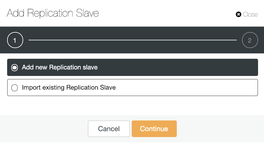
Let's see how adding a new replication slave can be a really easy task.
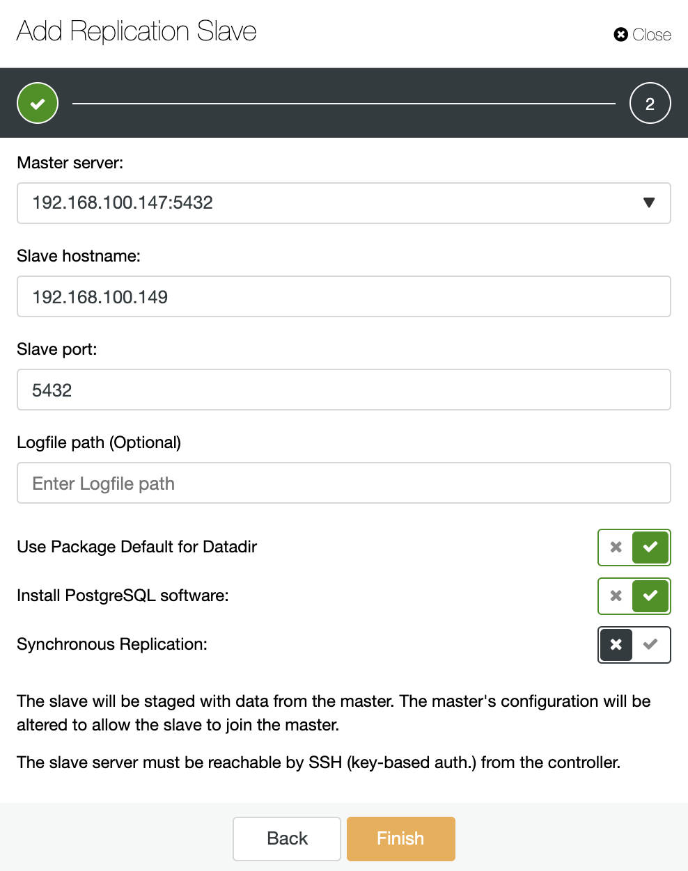
As you can see in the image, we only need to choose our Master server, enter the IP address for our new slave server and the database port. Then, we can choose if we want ClusterControl to install the software for us and if the replication slave should be Synchronous or Asynchronous.
In this way, we can add as many replicas as we want and spread read traffic between them using a load balancer, which we can also implement with ClusterControl.
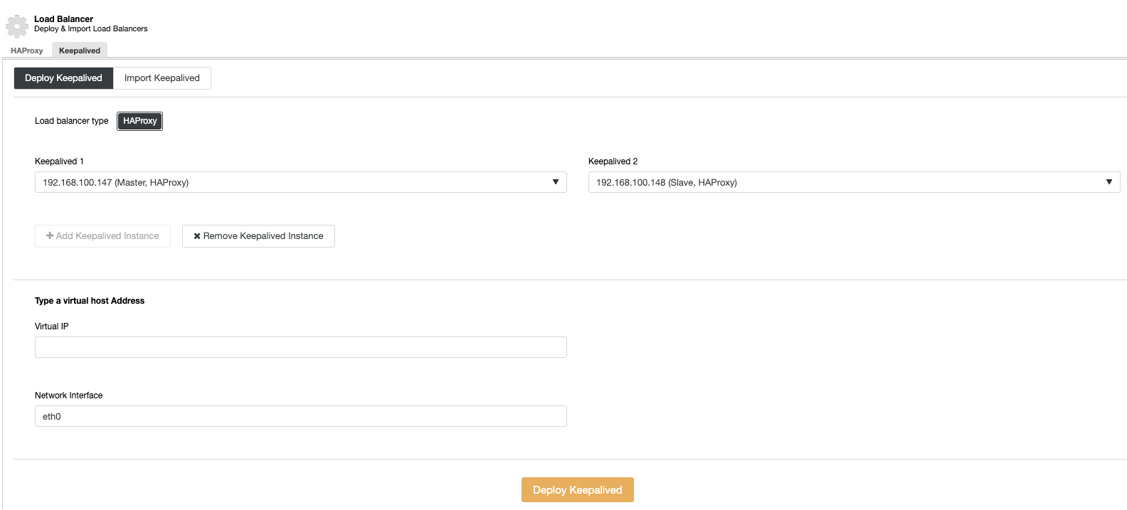
Now, if we go to cluster actions and select “Add Load Balancer”, we can deploy a new HAProxy Load Balancer or add an existing one.
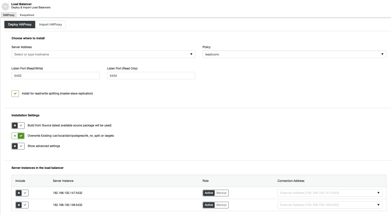
And then, in the same load balancer section, we can add a Keepalived service running on the load balancer nodes for improving our high availability environment.
Vertical Scaling
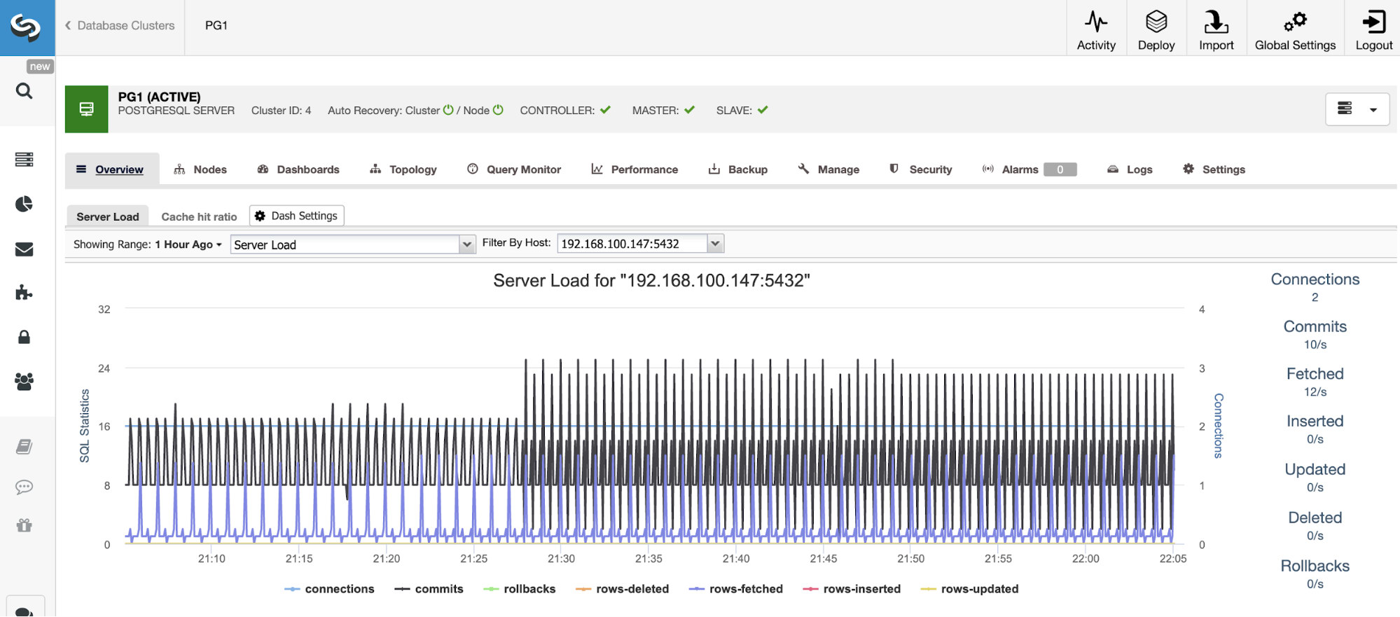
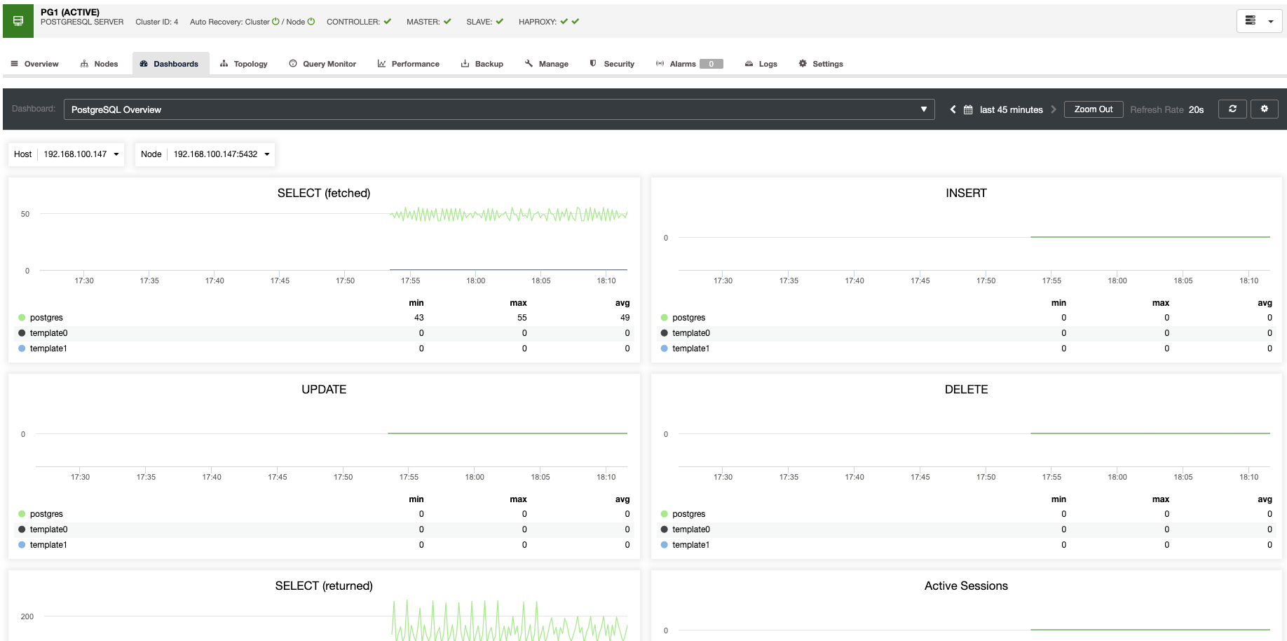
For vertical scaling, with ClusterControl we can monitor our database nodes from both the operating system and the database side. We can check some metrics like CPU usage, Memory, connections, top queries, running queries, and even more. We can also enable the Dashboard section, which allows us to see the metrics in more detailed and in a friendlier way our metrics.
From ClusterControl, you can also perform different management tasks like Reboot Host, Rebuild Replication Slave or Promote Slave, with one click.
Conclusion
Scaling our PostgreSQL database can be a time consuming task. We need to know what we need to scale and what the best way is to do it. As we could see, there are some metrics to take into account at time to scale it and they can help to know what we need to do.
ClusterControl provides a whole range of features, from monitoring, alerting, automatic failover, backup, point-in-time recovery, backup verification, to scaling of read replicas. This can help us to scale our PostgreSQL database in a horizontal or vertical way from a friendly and intuitive UI.
↧
Luca Ferrari: Checking PostgreSQL Version in Scripts
psql(1) has a bar support for conditionals, that can be used to check PostgreSQL version and act accordingly in scripts.
Checking PostgreSQL Version in Scripts
psql(1) provides a little support to conditionals and this can be used in scripts to check, for instance, the PostgreSQL version.
This is quite trivial, however I had to adjust an example script of mine to act properly depending on the PostgreSQL version.
The problem
The problem I had was with declarative partitioning: since PostgreSQL 11, declarative partitioning supports a DEFAULT partition, that is catch-all bucket for tuples that don’t have an explicit partition to go into. In PostgreSQL 10 you need to manually create catch-all partition(s) by explicitly defining them.
In my use case, I had a set of tables partitioned by a time range (the year, to be precise), but I don’t want to set up a partition for each year before the starting point of clean data: all data after year 2015 is correct, somewhere there could be some dirty data with bogus years.
Therefore, I needed a partition to catch all bogus data before year 2015, that is, a partition that ranges from the earth creation until 2015. In PostgreSQL 11 this, of course, requires you to define a DEFAULT partition and that’s it! But how to create a different default partition on PostgreSQL 10 and 11?
I solved the problem with something like the following:
\if:pg_version_10\echo'PostgreSQL version is 10'\echo'Emulate a DEFAULT partition'CREATETABLEdigikam.images_oldPARTITIONOFdigikam.images_rootFORVALUES ↧
Konstantin Evteev: Standby in production: scaling application in second largest classified site in the world.
Standby in production: scaling application in the second largest classified site in the world

Hi. My name is Konstantin Evteev, I’m a DBA Unit Leader of Avito. Avito is the biggest Russian classified site, and the second largest classified site in the world (after Craigslist of USA). Items offered for sale on Avito can be brand new or used. The website also publishes job vacancies and CVs.
Via its web and mobile apps, the platform monthly serves more than 35 million users. They add approximately a million new ads a day and close over 100,000 transactions per day. The back office has accumulated more than a billion ads. According to Yandex, in some Russian cities (for example, in Moscow), Avito is considered a high load project in terms of page views. Some figures can give a better idea of the project’s scale:
- 600+ servers;
- 4.5 Gbit/sec TX, 2 Gbit/sec RX without static;
- about a million queries per minute to the backend;
- 270TB of images;
- >20 TB in Postgres on 100 nodes:
- 7–8K TPS on most nodes;
- the largest — 20k TPS, 5 TB.
At the same time, these volumes of data need not only to be accumulated and stored but also processed, filtered, classified and made searchable. Therefore, expertise in data processing is critical for our business processes.
The picture below shows the dynamic of pageviews growth.
Our decision to store ads in PostgreSQL helps us to meet the following scaling challenges: the growth of data volume and growth of number of requests to it, the scaling and distribution of the load, the delivery of data to the DWH and the search subsystems, inter-base and internetwork data synchronization, etc. PostgreSQL is the core component of our architecture. Reach set of features, legendary durability, built-in replication, archive, reserve tools are found a use in our infrastructure. And professional community helps us to effectively use all these features.
In this report, I would like to share Avito’s experience in different cases of standby usage in the following order:
- a few words about standby and its history in general;
- problems and solutions in replication based horizontal scale-out;
- Avito’s implementation for solution to avoid stale reads from replica;
- possible pitfalls while using standby with high request rate, applying DDL, receiving WAL files from the archive;
- handling issues with technique of using several standbys in production and routing queries between them;
- logical replication based scaling example to compare;
- conclusions and standby major upgrade features.
A few words about standby and its history in general
Standby can be used for the following purposes.
- High availability: if primary crashes you need to have hot reserve to make fast failover
- Scaling — you can switch part or all your read queries between one or more standbys
In early 2000s, PostgreSQL community didn’t think that replication should be a built-in feature. Vadim Mikheev after implementation of MVCC, developed a replication solution «Rserv» based on MVCC internal mechanics. The following logic was supposed to be used to replicate data: taking changes that were not visible in a previous snapshot and became visible in the current snapshot. Then Jan Wieck developed an enterprise logical replication solution based on Vadim Mikheev’s idea and named it Slony (Russian for “elephant”) as a reverence for its author. Then the team from Skype created SkyTools with PgQ (the transactional queue) and Londiste (the logical replication solution based on PgQ). PostgreSQL 8.3 аdd several txid_*() functions to query active transaction IDs. This is useful for various replication solutions. (Jan). And finally Logical replication became a built-in feature in PostgreSQL 10.
Meanwhile, built-in binary replication was evolving.
- 2001 PostgreSQL 7.1: write-ahead log is created to improve write performance.
- 2005 PostgreSQL 8.0: point in time recovery, makes it possible to create handmade replication scripts to have warm reserve.
- 2008 PostgreSQL 8.3: administration of previously released warm standby feature (2006) becomes easier. That’s why someone still uses PostgreSQL 8.3 in production.
- 2010 PostgreSQL 9.0: since this version PostgreSQL standby has been able to serve read queries (hot standby), moreover release of streaming replication feature has simplified setting up replication and decreased possible replication lag.
- 2011 PostgreSQL 9.1: synchronous replication makes it easier to support SLA for applications working with critical data (for example information about financial transactions). Previously to avoid data loss you had to wait until your data was successfully replicated to standby or had to save data in two databases manually.
- 2013 PostgreSQL 9.3: standby can follow timeline switch which makes failover procedures easier.
- 2014 PostgreSQL 9.4: replication slots make it safer to setup standby without archive, but as a result standby fail can lead to master fail. Logical decoding becomes the fundament for built-in logical replication.
- 2016 PostgreSQL 9.6: multiple synchronous standbys give an opportunity to create more reliable clusters. Remote_apply makes it possible to serve read queries from standby without stale reads.
So we have discussed few classifications of standby: logical and physical, built-in and stand alone solutions, read only and not only read only, sync and async.
Now let’s look closer at physical built-in read only async standbу.
In Streaming Replication, three kinds of processes work together. A walsender process on the primary server sends WAL data to а standby server; and then, a walreceiver and startup processes on standby server receives and replays these data. A walsender and a walreceiver communicate using a single TCP connection.
Problems and solutions in replication based horizontal scale-out
When you use asynchronous standby, it can fall behind the primary. That’s why different rules for routing read queries to the primary or to the standby match different types of applications.
- First approach — don’t use any routing technique, just route any read query to standby. For some applications it will be good due to many reasons such as:
- low replication lag;
- specific profile of queries with a lack of or a small number of errors connected with stale reads;
- and so on.
But I don’t like this approach, let’s look at better techniques for routing read queries to standby.
2. Sometimes there is a specific business logic that can allow exploiting stale reads. For example, few years ago on Avito there was a 30-minute interval before our users could see new ads (time for anti-fraud check and other restrictions). So we successfully use this specific business rule for routing your read queries for other people’s ads. At the same time we route read queries to your own ads to the primary. Thus, you may edit your own ad and work with the actual ad’s state. To make this routing approach work in a correct way we need to support a replication lag lower than the 30-minute interval.
3. There can be situations when stale reads are not acceptable, even more interesting when you need to use few standbys to achieve a greater level of scale. To deal with them you need to use special techniques. Let’s look closer at our example and the technique to avoid stale reads
Avito’s implementation to avoid stale reads from replica
We successfully used the logical routing technique (number 2: based on business specific logic) when we faced the following spikes. In the picture you can see a diagram with the Load Average on a 28-physical-core machine (2X Intel(R) Xeon(R) CPU E5–2697 v3 @ 2.60GHz). When we started using Hyper-threading, we benchmarked and found out that most of our queries were successfully scaled with enabling Hyper-threading. But then the distribution of queries changed and the result of this can be seen on the diagram. When the level of load average got closer to the number of physical cores, the spikes happened.
The same spikes were observed on the CPU diagram below. From my side, I saw that all queries started being executed dozens of times longer.
So I experienced the capacity problem of the primary server. Actually, the capacity of one server is bounded by the most powerful market offering. If it does not fit you, it is a capacity problem. Normally, changing the architecture of your application is not so that fast and moreover it might be complicated and take a lot of time. Being under such circumstances I had to find a quick solution. As you can notice that the spikes are gone, we coped with the capacity problem by switching more read queries to standby (you can see the number of queries on standby on the following TPS diagram).
We distributed load among more nodes in the system by re-routing queries that don’t need to run on the primary. The main challenges in spreading read queries to replicas are stale reads and race conditions.
On the links you can see detailed description of routing reads based on replica WAL position technique. The main idea is to store the last committed LSN for the entity on which mutating request was executed. Then, when we subsequently want to fulfill a read operation for the same entity, we’ll check which replicas have consumed to that point or beyond it, and randomly select one from the pool. If no replicas are sufficiently advanced (i.e. say a read operation is being run very closely after the initial write), we’ll fall back to the master. Stale reads become impossible regardless of the state of any given replica.
We made some simplification in the technique above. We didn’t use exactly the same one because we didn’t have enough time and resources to rewrite application by implementing sticky connections based on LSN tracking.
At that time we were facing the capacity problem of the primary server, we had a huge monolithic application (it was in progress of splitting to microservice architecture). So it had a lot of complicated logic and deep nested calls — which forced us to make migration to sticky LSN sessions unreachable in short term period. But on the other hand, we had some historical background: we had a timestamp column in the user and the item tables (our main entities), which we filled with the help of PostgreSQL function now(): current date and time — start of current transaction. So we decided to use timestamp instead of LSN. Probably you know that timestamp can’t be used for the task of serialization data operations (or tracking position of replica in relation to primary) in PostgreSQL. To make this assumption we used the following arguments:
- we didn’t have long transactions (all of them lasted several milliseconds);
- we routed all read queries for the entity on which mutating request was executed within 7.5 minutes to primary server;
- we could route read queries to replicas, which must not fall behind in relation to primary greater than 5-minute interval.
Eventually, we came up with the following solution (we called it Avito Smart Cache). We replaced our cache based on Redis with the one implemented in Tarantool. (Tarantool is a powerful fast data platform that comes with an in-memory database and an integrated application server).
We made two levels of cache. The first level — the hot cache — stores sticky sessions. Sticky connections are supported by storing the timestamp of last user’s data mutation. Each user is given its own key so that the actions of one user would not lead to all other users being affected.
Let’s look closer at the approach we used to deliver user’s timestamp information to Tarantool. We have made some changes in our framework for working with database: we have added «on commit hook». In this «hook» we invoke sending data mutation’s timestamp to the 1st level of cache. You may notice, that there is a possibility when we successfully have made changes in PostgreSQL database but couldn’t deliver this info to cache (for example there was a network problem or application error or smth else). To deal with such cases we have made the Listener. All mutations on the database side are sent to the Listener using PostgreSQL LISTEN and NOTIFY features. Also, the Listener tracks last_xact_replay_timestamp of standby and has HTTP API from which Tarantool takes this information.
The second level is the cache for our read data to minimize utilization of PostgreSQL resources (replacing the old cache in Redis).
Some special features:
- On the schema there are 16 Tarantool shards to help us to be resilient. When 1 shard crashes, PostgreSQL can continue processing 1/16 queries without help of the cache.
- Decreasing the value of time interval used for routing queries causes the growth in number of queries to standby. Meanwhile, this leads to increasing probability that standbys lag is greater than the routing interval. If this happens, all queries will be sent to the primary server and it’s highly likely that the primary won’t be able to process all these requests. And this elicits one more fact: when you use 2 nodes (primary and standby in production), you need at least the 3rd node (2nd standby) for the reserve purpose, and there should be a disaster recovery plan for all parts of this complex infrastructure.
The main logic of working with smart cache is as follows.
Trying to find data on the main level of the cache, if we find it, it is success. If we do not then we try to get data on the 1st level hot cache. If we find data in the hot cache, it means that there were recent changes in our data and we should get data from primary.
Or if the standbys lag is greater than routing interval — we also should get data from the primary.
Otherwise, data hasn’t been changed for a long time and we can route read request to standby.
You may notice different ttl values — they are different because there is a probability of races and In cases where the probability is greater I use smaller ttl to minimize losses.
Thus we successfully implemented one of the techniques for routing queries and made eventually synchronized cache. But on the graph below you may notice the spikes. These spikes appeared when standby started falling behind due to some reasons such as different locks or specific profile of utilizing hardware resources. In the following part of my report, I would like to share Avito’s experience in solving those issues on the standbys.
Сases highlighting possible problems while using standby with high request rate, applying DDL, receiving WAL files from archive and handling some issues with technique of using few standbys in production and routing queries between them
1st: Deadlock on standby
Step 1:
The Infrastructure for this case is as follows:
- primary (master);
- standby;
- two tables: the items and the options.
Step 2
Open transaction on the primary and alter the options table.
Step 3
On the standby execute the query to get data from the items table.
Step 4
On the primary side alter the items table.
Step 5
Execute the query to get data from the items table.
In PostgreSQL versions lower than 10 we have a deadlock that is not detected. Such deadlocks have successfully been detected by deadlock detector since PostgreSQL 10.
2nd: DDL (statement_timeout and deadlock_timeout)
The infrastructure for this case is the same.
How to apply DDL changes to the table, receiving thousands read requests per second. Of course with the help of statement_timeout setting (Abort any statement that takes more than the specified number of milliseconds, starting from the time the command arrives at the server from the client. ).
Another setting you should use to apply DDL is deadlock_timeout. This is the amount of time, in milliseconds, to wait on a lock before checking to see if there is a deadlock condition. The check for deadlock is relatively expensive, so the server doesn’t run it every time it waits for a lock. We optimistically assume that deadlocks are not common in production applications and just wait on the lock for a while before checking for a deadlock. Increasing this value reduces the amount of time wasted in needless deadlock checks, but slows down reporting of real deadlock errors. The default is one second (1s), which is probably about the smallest value you would want in practice. On a heavily loaded server you might want to raise it. Ideally the setting should exceed your typical transaction time, so as to improve the odds that a lock will be released before the waiter decides to check for deadlock.
Deadlock timeout setting controls the time when conflicting autovacuum is canceled, because the default 1-second value is also the value of duration of the lock while applying DDL and it can lead to a trouble in systems with thousands requests per second.
There is some specifics in the scope of statement_timeout setting and the changes take effect ( for example changing statement_timeout inside the stored procedure will take no effect on this procedure call).
With the help of the settings above we repeatedly try to apply changes to the structure of our tables with a short lock (approximately dozens of ms). Sometimes we can’t do this (take a lock within dozens of ms) during the daytime, and then we try to do it at night, when the traffic rate is lower. Usually we manage to do it. Otherwise we increase the values of those settings(«time window» for getting the lock).
After execution of the DDL statement with timeouts on the primary, these changes are replicated to standby. Timeouts aren’t replicated to the standby that’s why there may be locks between the WAL replay process and read queries.
2018–01–12 16:54:40.208 MSK pid=20949,user=user_3,db=test,host=127.0.0.1:55763 LOG: process 20949 still waiting for AccessShareLock on relation 10000 of database 9000 after 5000.055 ms
2018–01–12 16:54:40.208 MSK pid=20949,user=user_3,db=test,host=127.0.0.1:55763 DETAIL: Process holding the lock: 46091. Wait queue: 18639, 20949, 53445, 20770, 10799, 47217, 37659, 6727, 37662, 25742, 20771,
We have implemented the workaround to deal with the issue above. We use the proxy to route queries to one of two standbys. And when we want to apply the DDL command on the primary, we stop replaying of the replication on the standby where the queries are executed.
- Wait till the ALTER command is replayed on the second standby.
- Then switch traffic to the second standby (which has successfully replayed the WAL with DDL statement).
- Start the replication on the first standby and wait till the ALTER command has been replayed on it.
Return the first standby to the pool of active standbys.
3rd: Vacuum replaying on standby and truncating data file
Vacuum can truncate the end of data file — the exclusive lock is needed for this action. At this moment on the standby long locks between read only queries and recovery process may occur. It happens because some unlock actions are not written to WAL. The example below shows a few AccessExclusive locks in one xid 920764961, and not a single unlock… Unlock happens much later. When the standby replays the commit.
The solution for that issue can be like:
- skip table truncation at VACUUM is coming in PostgreSQL 12;
- decrease the number of locks on standby (Postgres Professional idea).
In our case (when we faced problem above) we have a kind of table with logs. Almost append only — once a week we executed a delete query with timestamp condition, we cleaned records older than 2 weeks. This specific workload makes it possible to truncate the end of the data files with the autovacuum process. At the same time we actively use the standby for reading queries. The consequences can be seen above. Eventually we successfully solved that issue by executing cleaning queries more frequently: every hour.
4th: Restoring WAL from archive
On Avito we actively use standbys with the replication being set up with the help of an archive. This choice was made to have an opportunity to recreate any crashed node ( primary or standby) from the archive and then set it in a consistent state in relation to the current primary.
In 2015, we faced the following situation: some of our services started generating too many WAL files. As a result our archive command reached up the performance limits, you may notice the spikes with pending WAL files for sending to the archive on the graph below.
You can notice the green arrow pointing to the area, where we solved this issue. We implemented multithreaded archive command.
You can make a deep dive into the implementation following the github link. In short, it has the following logic: if the number of ready WAL files is lower than the threshold value, then the archive is to be done with one thread, else turn on a parallel archive technique.
But then we were faced the problem of CPU utilization on the standby. It was not obvious at first view that we were monitoring CPU utilization for our profile of load in a wrong way. Getting /proc/stat values we can see just a snapshot of the current CPU utilization. Archiving one WAL file in our case takes 60 ms and on the snapshots we don’t see the whole picture. The details could be seen with the help of the counter measurements.
Due to the above reasons there was a challenge for us to find the true answer why the standby was falling behind in relation to the primary (almost all standby CPU resources were utilized by archiving and unarchiving WAL files). The green arrow on the schema above shows the result of the optimization in the standby CPU usage. This optimization was made in a new archive schema, by delegating the archiving command execution to the archive server.
First let’s look under the hood of the old archive schema. The archive is mounted to the standby with the help of NFS. The primary sends the WAL files to archive through the standby (on this standby users’ read queries are routed to minimize the replication lag). The archive command includes the compression step, and it is carried out by the CPU of the standby server.
New archive schema:
- Compression step is carried out by the archive server CPU.
- Archive is not the single point of failure. WAL is normally archived in two archives, or at least in one (in case another one is crashed or becomes unavailable). Running synchronizing WAL files procedure after each backup is the way to deal with temporary unavailability of one of two archives servers.
- With the help of new archive schema we expanded the interval for PITR and the number of backups. We use the archives in turn, for example, 1st backup on 1st archive, 2nd backup on 2nd archive, 3rd backup on 1st archive, 4th backup on 2nd archive.
Both archive solutions were ideas of Michael Tyurin further developed by Sergey Burladyan and implemented by Victor Yagofarov. You can get it here. The solutions above were made for PostgreSQL versions where pg_rewind and pg_receivexlog were not available. With its help it is easier to deal with crashes in the distributed PostgreSQL infrastructure based on asynchronous replication. You can see the example of a crash of the primary at the schema below and there can be variants:
- some changes have been transferred neither to the standby nor to the archive;
- all the data has been transferred either to the standby or to the archive. In other words, the archive and the standby are in different states.
So there can be different cases with many «IFs» in your Disaster Recovery Plan. On the other hand, when something goes wrong it is harder to concentrate and to do everything right (for example). That’s why DRP must be clear to responsible stuff and be automated. There is a really beneficial report named «WARM standby done right» by Heikki Linnakangas where you can find a good overview and description of the tooling and the techniques to make warm standby.
Besides I want to share one configuration example of PostgreSQL infrastructure from my experience. Even using synchronous replication for standby and archive, it may happen that the standby and the archive are in different states after a crash of the primary. Synchronous replication works in such a manner: on the primary changes are committed, but there is a data structure in memory(it is not written to the WAL) that indicates that clients can’t see these changes. That indicator is stored until synchronous replicas send acknowledgment that they have successfully replayed the changes above.
Standbys pool
The existence of the possible lag of standby and other problems I have described above made us use the standbys pool in Avito’s infrastructure.
With the help of HAProxy and check function, we altered few standbys. The idea is that when the standby lag value is greater than the upper border, we close it for users’ queries until the lag value is smaller than the lower border.
if master
then false
if lag > max
then create file and return false
if lag > min and file exists
then return false
if lag < min and file exists
then remove file and return true
else
true
To implement this logic we need to make a record on the standby side. It can be implemented with the help of foreign data wrapper or untrusted languages(PL/Perl, PL/Python and etc).
Logical replication as an alternative tool to scale application
It is out of the current topic but I want to say that there is logical replication as an alternative of binary replication. With its help, the following Avito’s issues are successfully solved: the growth of data volume and growth of number of requests to it, the scaling and the distribution of the load, the delivery of data to the DWH and to the search subsystems, inter-base and intersystem data synchronization, etc. Michael Tyurin (ex chief architect) is the author of the majority of core solutions mentioned above, implemented with the help of SkyTools.
Both kinds of replication solutions have their strengths and weaknesses. Since PostgreSQL 10 logical replication has been a built-in feature. Andhere is an article with Avito’s recovery cases and techniques.
One of successful examples of logical replication usage in Avito is the organization of search results preview (since 2009 to the 1st quarter 2019). The idea is in making trigger-based materialized view (www.pgcon.org/2008/schedule/attachments/64_BSDCan2008-MaterializedViews-paper.pdf, www.pgcon.org/2008/schedule/attachments/63_BSDCan2008-MaterializedViews.pdf ), and then replicating it to another machine for read queries.
This Machine is much cheaper than the main server. And as a result, we serve all our search results from this node. On the graph below you can find information about TPS and CPU usage: it is very effective pattern of scale read load.
There are a lot more things to discuss such as reserve for logical replica, unlogged tables to increase performance, pros and cons and so on. But it is a completely different story and I will tell it next time. The point I want to highlight is that using logical replication can be very useful in many cases. There are no such drawbacks as in streaming replication, but it also has its own operation challenges. As a result there is no «silver bullet», knowledge about both types of replication helps us make the right choice in a specific case.
Conclusions
There are a few types of standby and each fits a specific case. When I was going to start preparing this report I intended to make the following conclusion. There are many operation challenges, that’s why it is better to scale your application with sharding. With the help of standby these tasks can be done without extra efforts:
- hot reserve;
- analytical queries;
- read queries when stale reads is not a problem.
Moreover, I was going to stop using binary standby for reading queries in Avito production. But opportunities have changed and we are going to build multi-datacenter architecture. Each service should be deployed at least in 3 datacenters. This is how the deploy schema looks like: a group of instances of each microservice and one node of its database (primary or standby) should be located in each data center. Reads will be served locally whereas writes will be routed to the primary.
So the opportunities make us use standby in production.
I have described several approaches and techniques above how to serve reads from standby. There are some pitfalls and a few of them have been found and successfully solved by us. Built-in solutions for pitfalls mentioned in this report could make standby operating experience better. For example, some kind of hints to write deadlock and statement timeout to WAL. If you are aware of other pitfalls let’s share that knowledge with us and the community.
Another crucial moment — is to make backups and reserve right way. Create your disaster recovery plan, support it in actual state with regular drills. Moreover, in order to minimize downtime period automize your recovery. One more aspect about reserve and standby is that if you use standby in production to execute application queries you should have another one for reserve purposes.
Suppose you have to do major upgrade and you can’t afford a long downtime. With primary and standby in production there is a high probability that one node can’t serve all queries (after the upgrade you should also have two nodes). To do this fast you can either use logical replication or upgrade master and standby with pg_upgrade. On Avito we use pg_upgrade. From the documentation, it is not obvious how to do it right if your standby receives WAL files from archive. If you use Log-Shipping standby servers (without streaming), the last file in which shutdown checkpoint record is written won’t be archived. To make the standby servers caught up you need to copy the last WAL file from primary to the standby servers and wait till it is applied. After that standby servers can issue restart point at the same location as in the stopped master. Alternatively, you can switchfrom Log-Shipping to Streaming Replication.
Yet another useful example from my upgrade experience.
In production config vacuum_defer_cleanup_age = 900000. With this setting pg_upgrade cannot freeze pg_catalog in a new cluster (it executes ‘vacuumdb — all — freeze’) during performing upgrade and upgrade fails:
Performing Upgrade
------------------
Analyzing all rows in the new cluster ok
Freezing all rows on the new cluster ok
Deleting files from new pg_clog ok
Copying old pg_clog to new server ok
Setting next transaction ID and epoch for new cluster ok
Deleting files from new pg_multixact/offsets ok
Copying old pg_multixact/offsets to new server ok
Deleting files from new pg_multixact/members ok
Copying old pg_multixact/members to new server ok
Setting next multixact ID and offset for new cluster ok
Resetting WAL archives ok
connection to database failed: FATAL: database "template1" does not exist
could not connect to new postmaster started with the command:
"/home/test/inst/pg9.6/bin/pg_ctl" -w -l "pg_upgrade_server.log" -D "new/"
-o "-p 50432 -b -c synchronous_commit=off -c fsync=off -c
full_page_writes=off -c listen_addresses='' -c unix_socket_permissions=0700
-c unix_socket_directories='/home/test/tmp/u'" start
Failure, exiting
Test script:
#!/bin/bash
PGOLD=~/inst/pg9.4/bin
PGNEW=~/inst/pg9.6/bin
${PGOLD}/pg_ctl init -s -D old -o "--lc-messages=C -T pg_catalog.english"${PGNEW}/pg_ctl init -s -D new -o "--lc-messages=C -T pg_catalog.english"echo vacuum_defer_cleanup_age=10000 >> new/postgresql.auto.conf
# move txid to 3 000 000 000 in old cluster as in production
${PGOLD}/pg_ctl start -w -D old -o "--port=54321--unix_socket_directories=/tmp"
${PGOLD}/vacuumdb -h /tmp -p 54321 --all --analyze${PGOLD}/vacuumdb -h /tmp -p 54321 --all --freeze${PGOLD}/pg_ctl stop -D old -m smart#
${PGOLD}/pg_resetxlog -x 3000000000 olddd if=/dev/zero of=old/pg_clog/0B2D bs=262144 count=1
# # move txid in new cluster bigger than vacuum_defer_cleanup_age may fix
problem
# ${PGNEW}/pg_ctl start -w -D new -o "--port=54321--unix_socket_directories=/tmp"
# echo "select txid_current();" | ${PGNEW}/pgbench -h /tmp -p 54321 -n -P 5-t 100000 -f- postgres
# ${PGNEW}/pg_ctl stop -D new -m smart${PGNEW}/pg_upgrade -k -d old/ -D new/ -b ${PGOLD}/ -B ${PGNEW}/# rm -r new old pg_upgrade_* analyze_new_cluster.sh delete_old_cluster.sh
I did not find any prohibition in the documentation on using production config with pg_upgrade, maybe I am wrong and this has already been mentioned in the documentation.
I and my colleagues are hoping to see improvements in replication in future PostgreSQL versions. Both replication approaches in PostgreSQL are a great achievement, it is very simple today to set up replication with high performance. This article is written to share Avito experience and highlight main demands of Russian PostgreSQL community (I suppose that members of PostgreSQL community worldwide face the same problems).
Standby in production: scaling application in second largest classified site in the world. was originally published in AvitoTech on Medium, where people are continuing the conversation by highlighting and responding to this story.
↧
Jeff McCormick: Using the PostgreSQL Operator with Rook Ceph Storage

The Crunchy PostreSQL Operator supports various forms of storage for provisioning PostgreSQL clusters in a Kubernetes environment. One such provider is Rook, which provides an abstract layer around multiple storage systems available in Kubernetes, which makes it even more convenient to choose between multiple storage engines. One storage engine that Rook supports is Ceph, which provides several types of distributed storage platforms including block-level storage, which is very helpful for expanding cloud-based workloads.
This post explores the use of the Rook storage engine with the PostgreSQL Operator, specifically demonstrating how the PostgreSQL Operator can be utilized to create a PostgreSQL cluster that is backed by Rook Ceph blockstorage.
For this example the rook-ceph-block storage class will be created and utilized in conjunction with the PostgreSQL Operator to dynamically provision Ceph block storage for use by a PostgreSQL cluster and it's supporting services. This will effectively demonstrate how Rook can be utilized to deploy a Ceph cluster in your Kubernetes environment, therefore allowing you to leverage the power of Ceph storage, e.g. highly-available and scalable block storage, in your PostgreSQL clusters.
Many thanks to Andrew L'Ecuyer for helping with the methodology and testing that this post presents. For more information about PostgreSQL Operator storage configuration, please see the documentation.

↧
↧
Stefan Fercot: pgBackRest S3 configuration
pgBackRest is a well-known powerful backup and restore tool.
While the documentation describes all the parameters, it’s not always that simple to imagine what you can really do with it.
In this post, I will introduce some of the parameters needed to configure the access to an Amazon S3 bucket.
MinIO
For the purpose of this demo setup, we’ll install a MinIO server, which is an Amazon S3 Compatible Object Storage.
To do so, I followed the guide of centosblog.com.
Installation
On a fresh CentOS 7 server:
$ sudo useradd -s /sbin/nologin -d /opt/minio minio
$ sudo mkdir -p /opt/minio/bin
$ sudo mkdir -p /opt/minio/data
$ sudo yum install -y wget
$ sudo wget https://dl.min.io/server/minio/release/linux-amd64/minio -O /opt/minio/bin/minio
$ sudo chmod +x /opt/minio/bin/minio
$ cat<<EOF | sudo tee "/opt/minio/minio.conf"
MINIO_VOLUMES=/opt/minio/data
MINIO_DOMAIN=minio.local
MINIO_OPTS="--certs-dir /opt/minio/certs --address :443 --compat"
MINIO_ACCESS_KEY="accessKey"
MINIO_SECRET_KEY="superSECRETkey"
EOF
$ sudo chown -R minio:minio /opt/minio
MinIO is installed in /opt/minio with a specific system user. The domain name
we’ll use will be minio.local and the bucket name will be pgbackrest.
The data will be stored in /opt/minio/data.
We then have to setup the hosts file accordingly:
$ cat<<EOF | sudo tee "/etc/hosts"
127.0.0.1 pgbackrest.minio.local minio.local s3.eu-west-3.amazonaws.com
EOF
Https
Since we’ll need to run MinIO in https mode to be able to work with pgBackRest, let’s create some self-signed certificates:
$ mkdir ~/certs
$ cd ~/certs
$ openssl genrsa -out ca.key 2048
$ openssl req -new-x509-extensions v3_ca -key ca.key -out ca.crt -days 99999 -subj"/C=BE/ST=Country/L=City/O=Organization/CN=some-really-cool-name"$ openssl genrsa -out server.key 2048
$ openssl req -new-key server.key -out server.csr -subj"/C=BE/ST=Country/L=City/O=Organization/CN=some-really-cool-name"$ openssl x509 -req-in server.csr -CA ca.crt -CAkey ca.key -CAcreateserial-out server.crt -days 99999 -sha256$ sudo mkdir -p-m 755 /opt/minio/certs
$ sudo cp server.crt /opt/minio/certs/public.crt
$ sudo cp server.key /opt/minio/certs/private.key
$ sudo chown -R minio:minio /opt/minio/certs
$ sudo chmod -R 644 /opt/minio/certs/public.crt
$ sudo chmod -R 644 /opt/minio/certs/private.key
$ cd ~
To show the accessKey and secretKey generated, use:
$ sudo grep-E'accessKey|secretKey' /opt/minio/data/.minio.sys/config/config.json
For this example, we’ve forced those values in the /opt/minio/minio.conf file.
Systemd
Create the systemd service:
$ cat<<EOF | sudo tee "/etc/systemd/system/minio.service"
[Unit]
Description=Minio
Documentation=https://docs.minio.io
Wants=network-online.target
After=network-online.target
AssertFileIsExecutable=/opt/minio/bin/minio

[Service]
AmbientCapabilities=CAP_NET_BIND_SERVICE
WorkingDirectory=/opt/minio

User=minio
Group=minio

PermissionsStartOnly=true

EnvironmentFile=-/opt/minio/minio.conf
ExecStartPre=/bin/bash -c "[ -n \\"\${MINIO_VOLUMES}\\" ] || echo \\"Variable MINIO_VOLUMES not set in /opt/minio/minio.conf\\""

ExecStart=/opt/minio/bin/minio server \$MINIO_OPTS \$MINIO_VOLUMES

StandardOutput=journal
StandardError=inherit

# Specifies the maximum file descriptor number that can be opened by this process
LimitNOFILE=65536

# Disable timeout logic and wait until process is stopped
TimeoutStopSec=0

# SIGTERM signal is used to stop Minio
KillSignal=SIGTERM

SendSIGKILL=no

SuccessExitStatus=0

[Install]
WantedBy=multi-user.target
EOF

$ sudo systemctl enable minio
$ sudo systemctl start minio
$ sudo firewall-cmd --quiet--permanent--add-service=https
$ sudo firewall-cmd --quiet--reload$ sudo systemctl status minio
Compared to the original service, I’ve added
AmbientCapabilities=CAP_NET_BIND_SERVICE to allow the service to start on
port 443. The firewall also allows the https access.
s3cmd
To create the pgbackrest bucket, we’ll use s3cmd. The package can be found
in the epel-release repositories.
$ sudo yum install -y epel-release
$ sudo yum --enablerepo epel-testing install -y s3cmd

$ cat<<EOF> ~/.s3cfg
host_base = minio.local
host_bucket = pgbackrest.minio.local
bucket_location = eu-west-3
use_https = true
access_key = accessKey
secret_key = superSECRETkey
EOF

$ s3cmd mb --no-check-certificate s3://pgbackrest
Bucket 's3://pgbackrest/' created
$ sudo mkdir /opt/minio/data/pgbackrest/repo
$ sudo chown minio: /opt/minio/data/pgbackrest/repo
$ s3cmd ls--no-check-certificate s3://pgbackrest/repo
                       DIR   s3://pgbackrest/repo/
We’ve also created a repo sub-directory that we’ll use to store
the pgBackRest files.
PostgreSQL and pgBackRest installation
Let’s install PostgreSQL and pgBackRest directly from the PGDG yum repositories:
$ sudo yum install -y https://download.postgresql.org/pub/repos/yum/11/redhat/\
rhel-7-x86_64/pgdg-centos11-11-2.noarch.rpm
$ sudo yum install -y postgresql11-server postgresql11-contrib
$ sudo yum install -y pgbackrest
Check that pgBackRest is correctly installed:
$ sudo-iu postgres pgbackrest
pgBackRest 2.15 - General help

Usage:
    pgbackrest [options] [command]

Commands:
    archive-get     Get a WAL segment from the archive.
    archive-push    Push a WAL segment to the archive.
    backup          Backup a database cluster.
    check           Check the configuration.
    expire          Expire backups that exceed retention.
    help            Get help.
    info            Retrieve information about backups.
    restore         Restore a database cluster.
    stanza-create   Create the required stanza data.
    stanza-delete   Delete a stanza.
    stanza-upgrade  Upgrade a stanza.
    start           Allow pgBackRest processes to run.
    stop            Stop pgBackRest processes from running.
    version         Get version.

Use 'pgbackrest help [command]'for more information.
Create a basic PostgreSQL cluster:
$ export PGSETUP_INITDB_OPTIONS="--data-checksums"$ sudo /usr/pgsql-11/bin/postgresql-11-setup initdb
Configure archiving in the postgresql.conf file:
$ cat<<EOF | sudo tee -a "/var/lib/pgsql/11/data/postgresql.conf"
archive_mode = on
archive_command = 'pgbackrest --stanza=my_stanza archive-push %p'
EOF
Start the PostgreSQL cluster:
$ sudo systemctl start postgresql-11
Configure pgBackRest to point to the S3 bucket
$ cat<<EOF | sudo tee "/etc/pgbackrest.conf"
[global]
repo1-path=/repo
repo1-type=s3
repo1-s3-endpoint=minio.local
repo1-s3-bucket=pgbackrest
repo1-s3-verify-ssl=n
repo1-s3-key=accessKey
repo1-s3-key-secret=superSECRETkey
repo1-s3-region=eu-west-3

repo1-retention-full=1
process-max=2
log-level-console=info
log-level-file=debug
start-fast=y
delta=y

[my_stanza]
pg1-path=/var/lib/pgsql/11/data
EOF
Finally, create the stanza and check that everything works fine:
$ sudo-iu postgres pgbackrest --stanza=my_stanza stanza-create
...
P00   INFO: stanza-create command end: completed successfully

$ sudo-iu postgres pgbackrest --stanza=my_stanza check
...
P00   INFO: WAL segment 000000010000000000000001 successfully stored...
P00   INFO: check command end: completed successfully
Let’s finally take our first backup:
$ sudo-iu postgres pgbackrest --stanza=my_stanza --type=full backup
...
P00   INFO: new backup label = 20190718-194303F
P00   INFO: backup command end: completed successfully
...
And that’s it! You’re ready to go! Enjoy, test it with a real Amazon S3 bucket
and don’t hesitate to perform some performance tests with, for example, pgbench.
pgBackRest configuration explanations
What the documentation says:
repo1-s3-endpoint
S3 repository endpoint.
The AWS end point should be valid for the selected region.
Remark: that’s why a good DNS resolution is needed!
repo1-s3-bucket
S3 repository bucket.
S3 bucket used to store the repository.
pgBackRest repositories can be stored in the bucket root by setting
repo-path=/ but it is usually best to specify a prefix, such as /repo, so
logs and other AWS generated content can also be stored in the bucket.
repo1-s3-verify-ssl
Verify S3 server certificate.
Disables verification of the S3 server certificate. This should only be used for testing or other scenarios where a certificate has been self-signed.
tl;dr: this option would be, I think, very useful in the official
Net::Amazon::S3 perl module…
repo1-s3-region
S3 repository region.
The AWS region where the bucket was created.
Conclusion
pgBackRest offers a lot of possibilities. As long as we use the default https port (443), we can use the S3 configurations with other S3 compatible API’s like MinIO. Pretty much useful, right?
↧
Hans-Juergen Schoenig: PostgreSQL: How are functions and stored procedures replicated?
When looking at our PostgreSQL support activities, we notice that people often ask about functions, stored procedures and replication. Are functions replicated? How are functions replicated? What happens to shared libraries and do we have to install an extension everywhere? This topic seems to be really interesting to many people and so I decided to write a small post about this issue to hopefully shed some light on it.
How PostgreSQL “stores” functions and procedures
To understand how PostgreSQL “replicates” functions, it is first important to understand how functions and procedures are actually stored. To demonstrate this, I have created a small function that just returns a number and quits:
test=# CREATE FUNCTION demo(int)
		RETURNS int AS
$$
	SELECT 1;
$$ 	LANGUAGE 'sql';
CREATE FUNCTION
PostgreSQL stores the code of a function in a system table. In case the function is written in an “interpreted” language, the code is just stored there in plain text. The following listing shows, how this works:
test=# SELECT proname, prolang, prokind, prosrc, probin
		FROM 	pg_proc
		WHERE proname = 'demo';
 proname | prolang | prokind |   prosrc    | probin
---------+---------+---------+-------------+--------
 demo    |      14 | f       |  SELECT 1;  |
(1 row)
What we see here is that “demo” has been written in language number 14 (which happens to be SQL), it is a “function” and not a procedure. Then there is the code of the function. Note that “probin” is empty – I will get back to that one a bit later. Now: What does that imply? If you use streaming replication (perhaps together with Patroni or some other tools) the system catalog will be replicated just like any other table. The function will therefore be sent to the remote side just like any other change. So the function will be fully replicated and there is nothing else to do.
Dealing with compiled stored procedure languages
What happens if you want to use compiled functions? – Maybe a stored procedure written in C, PostGIS or any other extension that was not written in SQL or PL/pgSQL.
Here is what happens:
test=# CREATE EXTENSION pg_trgm;
CREATE EXTENSION
test=# SELECT proname, prolang, prokind, prosrc, probin
		FROM 	pg_proc
		WHERE 	proname = 'show_trgm';
  proname  | prolang | prokind |  prosrc   |     probin
-----------+---------+---------+-----------+-----------------
 show_trgm |      13 | f       | show_trgm | $libdir/pg_trgm
(1 row)
To show how things work, I have enabled the pg_trgm extension that is shipped as part of PostgreSQL. What we see is that C code is not stored in prosrc. Instead, it contains the name of the function in the shared object listed in probin. If we add the extension and thus the function, the changes made to the system table are still replicated to your slaves just like any other change.
But: YOU have to ensure that the shared object is actually installed on the other side. It is not enough to install, say, PostGIS binaries on the master and magically hope that shared objects will be replicated too. That won’t happen and it never will.
It is important to mention: If you create a function on the master written in C and your slave does not have the desired library, the changes in the system tables will be present – there is just no way to call these functions on the slave.
Conclusion
Make sure that libraries are installed on all hosts in your cluster. Otherwise, things will break. PostgreSQL will replicate changes made to the system tables, but does not magically send libraries over the wire.
If you want to learn more about functions in PostgreSQL 12, check out our post about “optimizer support functions” right on our website.
The post PostgreSQL: How are functions and stored procedures replicated? appeared first on Cybertec.
↧
Michael Paquier: Postgres 12 highlight - Recovery changes
PostgreSQL 12 has changed the way recovery configuration works, and has introduced a couple of incompatible issues as mentioned in the main commit which has done the switch:
commit: 2dedf4d9a899b36d1a8ed29be5efbd1b31a8fe85
author: Peter Eisentraut <peter_e@gmx.net>
date: Sun, 25 Nov 2018 16:31:16 +0100
Integrate recovery.conf into postgresql.conf

recovery.conf settings are now set in postgresql.conf (or other GUC
sources).  Currently, all the affected settings are PGC_POSTMASTER;
this could be refined in the future case by case.

Recovery is now initiated by a file recovery.signal.  Standby mode is
initiated by a file standby.signal.  The standby_mode setting is
gone.  If a recovery.conf file is found, an error is issued.

The trigger_file setting has been renamed to promote_trigger_file as
part of the move.

The documentation chapter "Recovery Configuration" has been integrated
into "Server Configuration".

pg_basebackup -R now appends settings to postgresql.auto.conf and
creates a standby.signal file.

Author: Fujii Masao <masao.fujii@gmail.com>
Author: Simon Riggs <simon@2ndquadrant.com>
Author: Abhijit Menon-Sen <ams@2ndquadrant.com>
Author: Sergei Kornilov <sk@zsrv.org>
Discussion: https://www.postgresql.org/message-id/flat/607741529606767@web3g.yandex.ru/
From the point of view of code and maintenance, this has the huge advantage of removing the duplication caused by the parsing of recovery.conf which followed its own set of rules that were rather close to what is used for the generic GUC parameters, and this adds all the benefits behind GUCs, as it becomes possible:
- To reload parameters.
- To monitor the values with SHOW.
- To apply changes with ALTER SYSTEM.
However this introduces a set of compatibility changes to be aware of in order to adapt to the new rules.
First note that upgrading a standby instance to 12 and newer versions will cause an immediate failure, as the startup process would complain about the presence of recovery.conf:
FATAL:  using recovery command file "recovery.conf" is not supported
LOG:  startup process (PID 28201) exited with exit code 1
Here is a note about the backward-incompatible changes done:
- standby_mode has been removed from the parameters, and is replaced by an on-disk file called standby.signal as it represents a state of the cluster, so a configuration parameter does not map completely with its role.
- trigger_file is renamed to promote_trigger_file.
- pg_basebackup -R generated recovery.conf, and now all the parameters are written to postgresql.auto.conf instead which is used by ALTER SYSTEM by default.
In the background, nothing much changes as even if all the recovery-related values are available in the GUC context of a session, only the startup process makes use of it.
In the initial implementation, all the parameters were marked as PGC_POSTMASTER, meaning that they could just be loaded at server start time, and an update required a server restart to be effective. An additional improvements has made some of those parameters as reloadable, which is an upgrade compared to past versions of PostgreSQL. Here are the parameters concerned:
- archive_cleanup_command, to control the way past WAL segments are cleaned up, useful to control retention of the WAL archives depending on how much a standby feeds from it.
- promote_trigger_file, the file checked after to end recovery and promote a cluster as a new primary with a timeline bump.
- recovery_end_command. Note here that this command is only triggered once at the end of recovery, but it can be useful to update it on a set of standbys if migrating a configuration.
- recovery_min_apply_delay, which is very useful to tune the requests done to check when WAL is available, and when recovering from the archives this can be tuned dynamically to control the requests to a server where WAL archives are located.
There are plans to make more parameters reloadable, particularly primary_conninfo. This could not make it to PostgreSQL 12, and is much trickier than the others as this requires changes around the way a WAL receiver spawn request is done from the startup process.
↧
Luca Ferrari: yum upgrade postgresql11 panic!
I have to say, I don’t use CentOS very much and I’m not a good user of systemd, that is the reason why I got five minutes of pure fear!
yum upgrade postgresql11 panic!
How hard could it be to upgrade PostgreSQL within minor versions?
Usually it is very simple, and it is very simple but not when you don’t know your tools!
And in this case that’s my fault.
However, I’m writing this short note in order to avoid other people experience the same problem I had.
The current setup
The machine is a CentOS 7 running PostgreSQL 11.1 installed by packages provided by the PostgreSQL Global Development Group.
Preparing to upgrade
Of course, I took a full backup before proceeding, just in case. The cluster I’m talking about is a low traffice cluster with roughly ~12 GB~ of data, that is the backup and restore are not a zero downtime (and no, I’m not in the position of having a WAL based backup, but that’s another story).
Having a backup helps keeping the amount of panic at a fair level.
Performing the upgrade
I do like yum(8) and its transactional approach. Doing the upgrade was a matter of:
% sudo yum upgrade postgresql11 and all dependencies are, of course, calculated and applied. Then I confirmed, waited a couple of minutes for the upgrade to apply, and I started keeping my breath:
psql: could not connect to server: Connection refused Is the server running on host "xxx"(192.168.222.123) and accepting TCP/IP connections on port 5432? Inspecting and solving the problem
Apparently PostgreSQL has not been restarted after the upgrade,...
↧
↧
Jonathan Katz: Certificate Authentication Recipe for PostgreSQL Docker Containers

One of the reasons that PostgreSQL supports many authentication methods is to help ensure that it can work with multiple external identity management providers. While a lot of people are familiar with having PostgreSQL request a password for logging in, there are other
One method that can be used in larger enterprise environments is using certificates to authenticate between a PostgreSQL client (or user) and the server. Using certificates for authentication can have a lot of advantages, as they can provide a way to verify a user without requiring a password! In other words, you can avoid some of the challenges of having to secure shared passwords that are distributed across your infrastructure.
This articles on getting your own certificate-based authentication system set up in a PostgreSQL container with OpenSSL by going through the steps of setting up such a configuration and then exploring the extra variables you need to set in order to authenticate. If you're interested in setting up a production-level system, my colleague Stephen Frost gave an excellent talk at PGCon 2019 on how to set up an enterprise certificate-based authentication system (while also spending significant time on authenticating to PostgreSQL via the GSS-API and Kerberos),
tl;dr: What's the recipe?

↧
Avinash Kumar: Automatic Index Recommendations in PostgreSQL using pg_qualstats and hypopg

In my previous blog post, we have seen how the extension hypopg can be helpful in creating hypothetical indexes in PostgreSQL. If you have read it already, you know that it is very useful in verifying whether an Index can improve the performance of an SQL without having to create it in reality. Considering this, is there also a way to automatically suggest which indexes can improve the performance of some of your SQL’s? The answer is… YES!
In this blog post, we will see how we can get a direct recommendation to improve a specific query, as seen in the following snippet.
query                       |                 recmnded_index                 | percent_improvd
---------------------------------------------------+------------------------------------------------+-----------------
 select * from foo.bar where id2 = $1 and id4 = $2 | CREATE INDEX ON foo.bar USING btree (id2, id4) |           99.96
 select * from foo.bar where id3 = $1              | CREATE INDEX ON foo.bar USING btree (id3)      |           99.93
(2 rows)
Without any further delay, let’s discuss the extension
pg_qualstatswhich enables us to achieve this requirement for PostgreSQL versions 9.4 or later. Following that, we will take a look at a logic which could automatically suggest what indexes would be helpful for query optimizations – without much manual work.
All of the logic discussed in this blog post is reproducible, so please feel free to do so using the commands and try tuning your custom queries in test environments.
pg_qualstats
pg_qualstats is an extension developed by the POWA Team to uncover the need for storing predicates (quals). It stores the predicates found in WHERE clauses and JOIN conditions. This helps us analyze a query execution and opens up the possibility of automatic query optimizations.
When we query
pg_stat_statementslike extensions, we only see the prepared SQL or the SQL without any bind variable values. As you cannot perform an EXPLAIN (to see the execution plan of a Query) without the quals, the only option available is to see if that query was logged in the PostgreSQL log file and then identify the parameters passed to it. Or you can maybe use some arbitrary values, but this requires some manual intervention and time. But, when you create this extension: pg_qualstats, it stores queries along with the actual quals based on the sample rate (
pg_qualstats.sample_rate) specified.
Creating the extension: pg_qualstats
For RedHat/CentOS, we can install it using the packages available in the PGDG repository. Once you have added the PGDG repo, simply run the following command:
# yum install pg_qualstats11
Similarly for Ubuntu/Debian:
# apt install postgresql-11-pg-qualstats
Once installed, you must add
pg_qualstatsto
shared_preload_libraries. This requires a restart. As I am also using
pg_stat_statementsto get the
queryidassociated with each query recorded by
pg_qualstats, I have the following setting in my
postgresql.conffile:
shared_preload_libraries = 'pg_stat_statements, pg_qualstats'
Modifying the above parameter requires a restart of your PostgreSQL instance.
Some GUCs you should know
In order to start taking advantage of this extension, you may have to set some of the
GUCs(Grand Unified Configuration) in your PostgreSQL server. These can be set using
ALTER SYSTEMor by manually adding the associated entries in your
postgresql.confor
postgresql.auto.conffiles.
pg_qualstats.enabled: true or false (to enable or to disable pg_qualstats). ON by default.
pg_qualstats.track_constants: true or false (to enable tracking of each constant. False would reduce the number of entries to track predicates.)
pg_qualstats.max: The number of queries tracked. Defaults to 1000.
pg_qualstats.resolve_oids: Just store the oids or resolve them and store at query time. This takes additional space.
pg_qualstats.track_pg_catalog: Defaults to false. Whether or not the predicates of the objects in pg_catalog schema should be computed.
pg_qualstats.sample_rate: Default is -1. The fraction of queries to be sampled. -1 defaults to (1/max_connections). When set to 1, everything is sampled. Similarly when set to 0.1, one out of 10 queries are sampled.
Quals and Query Examples
In order to see this in action, let us use sysbench-tpcc to generate some SQL traffic, and then see some of the details captured.
Before running
sysbench-tpcc, I have created all the required extensions as seen in the following log. In order to see the
queryid(same as the
queryidcolumn of
pg_stat_statements) associated with each qual captured, it is important to have the extension:
pg_stat_statementscreated. Similarly, to create hypothetical indexes, we need to have the extension:
hypopgcreated.
percona=# CREATE EXTENSION hypopg;
CREATE EXTENSION
percona=# CREATE EXTENSION pg_stat_statements ;
CREATE EXTENSION
percona=# CREATE EXTENSION pg_qualstats;
CREATE EXTENSION
percona=# \dx
                                     List of installed extensions
        Name        | Version |   Schema   |                        Description
--------------------+---------+------------+-----------------------------------------------------------
 hypopg             | 1.1.3   | public     | Hypothetical indexes for PostgreSQL
 pg_qualstats       | 1.0.8   | public     | An extension collecting statistics about quals
 pg_stat_statements | 1.6     | public     | track execution statistics of all SQL statements executed
 plpgsql            | 1.0     | pg_catalog | PL/pgSQL procedural language
(4 rows)

percona=# show shared_preload_libraries ;
     shared_preload_libraries
----------------------------------
 pg_stat_statements, pg_qualstats
(1 row)
For this test, I have set
pg_qualstats.sample_rateto 1. Setting this to 1 captured every qual. We can, of course, reduce the sampling to ensure not everything is captured.
$ psql -d percona -c "ALTER SYSTEM SET pg_qualstats.sample_rate TO 1"
ALTER SYSTEM

$ psql -c "select pg_reload_conf()"
 pg_reload_conf
----------------
 t
(1 row)
Installing and running sysbench-tpcc on RedHat/CentOS
$ sudo yum install https://repo.percona.com/yum/percona-release-latest.noarch.rpm
$ sudo yum install git sysbench
$ git clone https://github.com/Percona-Lab/sysbench-tpcc.git
$ cd sysbench-tpcc
$ ./tpcc.lua --pgsql-user=postgres --pgsql-port=5432 --pgsql-db=percona --time=10 --threads=2 --report-interval=1 --tables=2 --scale=2 --use_fk=0  --trx_level=RC --db-driver=pgsql prepare
$ ./tpcc.lua --pgsql-user=postgres --pgsql-port=5432 --pgsql-db=percona --time=10 --threads=2 --report-interval=1 --tables=2 --scale=2 --use_fk=0  --trx_level=RC --db-driver=pgsql run
After running the benchmark for 10 seconds, we are now ready to query the view:
pg_qualstats_indexesthat gives us a nice view of the columns on which there are no indexes.
percona=# select * from pg_qualstats_indexes;
    relid    |   attnames   |      possible_types      | execution_count
-------------+--------------+--------------------------+-----------------
 customer2   | {c_id}       | {brin,btree,hash}        |               4
 customer2   | {c_last}     | {brin,btree,hash,spgist} |              33
 customer1   | {c_id}       | {brin,btree,hash}        |               7
 customer1   | {c_last}     | {brin,btree,hash,spgist} |               8
 orders2     | {o_c_id}     | {brin,btree,hash}        |               2
 order_line1 | {ol_o_id}    | {brin,btree}             |             208
 order_line2 | {ol_o_id}    | {brin,btree}             |             202
 order_line2 | {ol_o_id}    | {brin,btree,hash}        |              20
 stock1      | {s_quantity} | {brin,btree}             |             208
 stock2      | {s_quantity} | {brin,btree}             |             202
(10 rows)
Automatic Index Recommendations
In the previous section, we have seen the columns (of tables used in some of the SQLs in WHERE condition) which do not have indexes on them. Indexes on these columns can be considered as recommended indexes. To make this more meaningful, I have written the following function to store the queries that are using these columns as predicates, along with their execution plans
beforeand
aftercreating the recommended index. Using this data, we can understand whether the recommended index is really helpful.
CREATE OR REPLACE FUNCTION find_usable_indexes()
RETURNS VOID AS
$$
DECLARE
    l_queries     record;
    l_querytext     text;
    l_idx_def       text;
    l_bef_exp       text;
    l_after_exp     text;
    hypo_idx      record;
    l_attr        record;
    /* l_err       int; */
BEGIN
    CREATE TABLE IF NOT EXISTS public.idx_recommendations (queryid bigint,
    query text, current_plan jsonb, recmnded_index text, hypo_plan jsonb);
    FOR l_queries IN
    SELECT t.relid, t.relname, t.queryid, t.attnames, t.attnums,
    pg_qualstats_example_query(t.queryid) as query
      FROM
        (
         SELECT qs.relid::regclass AS relname, qs.relid AS relid, qs.queryid,
         string_agg(DISTINCT attnames.attnames,',') AS attnames, qs.attnums
         FROM pg_qualstats_all qs
         JOIN pg_qualstats q ON q.queryid = qs.queryid
         JOIN pg_stat_statements ps ON q.queryid = ps.queryid
         JOIN pg_amop amop ON amop.amopopr = qs.opno
         JOIN pg_am ON amop.amopmethod = pg_am.oid,
         LATERAL
              (
               SELECT pg_attribute.attname AS attnames
               FROM pg_attribute
               JOIN unnest(qs.attnums) a(a) ON a.a = pg_attribute.attnum
               AND pg_attribute.attrelid = qs.relid
               ORDER BY pg_attribute.attnum) attnames,
         LATERAL unnest(qs.attnums) attnum(attnum)
               WHERE NOT
               (
                EXISTS
                      (
                       SELECT 1
                       FROM pg_index i
                       WHERE i.indrelid = qs.relid AND
                       (arraycontains((i.indkey::integer[])[0:array_length(qs.attnums, 1) - 1],
                        qs.attnums::integer[]) OR arraycontains(qs.attnums::integer[],
                        (i.indkey::integer[])[0:array_length(i.indkey, 1) + 1]) AND i.indisunique)))
                       GROUP BY qs.relid, qs.queryid, qs.qualnodeid, qs.attnums) t
                       GROUP BY t.relid, t.relname, t.queryid, t.attnames, t.attnums
    LOOP
        /* RAISE NOTICE '% : is queryid',l_queries.queryid; */
        execute 'explain (FORMAT JSON) '||l_queries.query INTO l_bef_exp;
        execute 'select hypopg_reset()';
        execute 'SELECT indexrelid,indexname FROM hypopg_create_index(''CREATE INDEX on '||l_queries.relname||'('||l_queries.attnames||')'')' INTO hypo_idx;
        execute 'explain (FORMAT JSON) '||l_queries.query INTO l_after_exp;
        execute 'select hypopg_get_indexdef('||hypo_idx.indexrelid||')' INTO l_idx_def;
        INSERT INTO public.idx_recommendations (queryid,query,current_plan,recmnded_index,hypo_plan)
        VALUES (l_queries.queryid,l_querytext,l_bef_exp::jsonb,l_idx_def,l_after_exp::jsonb);
    END LOOP;
        execute 'select hypopg_reset()';
END;
$$ LANGUAGE plpgsql;
The above function uses the following logic:
- Create a Table with name:
public.idx_recommendations
where the results are stored. It stores the queries on which the table and column names mentioned in the output ofpg_qualstats_indexes
are used as predicates, along with their execution plan before and after creating thehypothethical
indexes. - Get the list of Queries (candidates for query tuning) along with their
queryid
and the attributes on which an index is recommended for each query. The SQL in the aboveFOR LOOP
is built using a slight modification to the existing view:pg_qualstats_indexes
.relid | relname | queryid | attnames | attnums | query -------+-------------+------------+------------+---------+-------------------------------------------- 17725 | customer2 | 297872607 | c_id | {1} | UPDATE customer2 .... 17725 | customer2 | 702831032 | c_id | {1} | UPDATE customer2 .... 17725 | customer2 | 1509701064 | c_last | {6} | SELECT count(c_id) namecnt .... 17725 | customer2 | 1539164311 | c_id | {1} | SELECT c_discount, c_last, c_credit, w_t 17725 | customer2 | 1976730265 | c_last | {6} | SELECT c_id FROM customer2 ...... 17725 | customer2 | 2041891134 | c_id | {1} | SELECT c_first, c_middle, c_last, c_stre.. 17728 | customer1 | 850567043 | c_id | {1} | SELECT c_first, c_middle, c_last, c_stre.. 17728 | customer1 | 977223112 | c_last | {6} | SELECT count(c_id) namecnt .... 17728 | customer1 | 2618115206 | c_id | {1} | SELECT c_discount, c_last, c_credit, w_t.. 17728 | customer1 | 2965820579 | c_last | {6} | SELECT c_id FROM customer1 .... 17728 | customer1 | 3738483437 | c_id | {1} | UPDATE customer1 .... 17752 | orders2 | 2217779140 | o_id | {1} | SELECT o_c_id .... 17752 | orders2 | 2709941400 | o_id | {1} | UPDATE orders2 .... 17762 | new_orders2 | 3012757930 | no_o_id | {1} | DELETE FROM new_orders2 .... 17771 | order_line2 | 192474146 | ol_o_id | {1} | SELECT COUNT(DISTINCT (s_i_id)) .... 17771 | order_line2 | 313117619 | ol_o_id | {1} | UPDATE order_line2 .... 17771 | order_line2 | 2921207531 | ol_o_id | {1} | SELECT SUM(ol_amount) sm .... 17782 | stock2 | 192474146 | s_quantity | {3} | SELECT COUNT(DISTINCT (s_i_id)) .... (18 rows) - An example query with predicates can be obtained using the function :
pg_qualstats_example_query()
provided bypg_qualstats
.percona=# select pg_qualstats_example_query(297872607); pg_qualstats_example_query ------------------------------------------------------------------------------- UPDATE customer2 + SET c_balance=-1576.000000, c_ytd_payment=1576.000000+ WHERE c_w_id = 2 + AND c_d_id=9 + AND c_id=900 (1 row) - Run
EXPLAIN
on the example query to store it in the table: public.idx_recommendations. - Use
hypopg
to create a hypothetical index on the attributes mentioned as columns without an index on them. - Run EXPLAIN on the query again and use
hypopg_reset()
to drop the hypothetical index created.
When I have validated if any of the queries generated by
sysbench-tpccneed some tuning using indexing, it was not a surprise that none of those need any further indexing. Hence, for the purpose of a demo, I have created a table and ran a few queries as following.
percona=# CREATE TABLE foo.bar (id int, dept int, id2 int, id3 int, id4 int, id5 int,id6 int,id7 int,details text, zipcode int);
CREATE TABLE
percona=# INSERT INTO foo.bar SELECT (random() * 1000000)::int, (random() * 1000000)::int, (random() * 1000000)::int,
(random() * 1000000)::int,(random() * 1000000)::int,(random() * 1000000)::int,(random() * 1000000)::int,(random() * 1000000)::int,
md5(g::text), floor(random()* (20000-9999 + 1) + 9999)
FROM generate_series(1,1*1e6) g;
INSERT 0 1000000
percona=# CREATE INDEX idx_btree_bar ON foo.bar (id, dept, id2,id3,id4,id5,id6,zipcode);
CREATE INDEX
percona=# select * from foo.bar where id2 = 1 and id4 = 3;
 id | dept | id2 | id3 | id4 | id5 | id6 | id7 | details | zipcode
----+------+-----+-----+-----+-----+-----+-----+---------+---------
(0 rows)
percona=# select * from foo.bar where id3 = 3;
   id   |  dept  |  id2   | id3 |  id4   | id5  |  id6   |  id7   |             details              | zipcode
--------+--------+--------+-----+--------+------+--------+--------+----------------------------------+---------
 876920 | 723557 | 670210 |   3 | 321924 | 9512 | 183549 | 756279 | 3e780bae1aacbebc10b1e06ca49d226e |   16364
(1 row)
Now, let us check if we can find the indexes that could improve the SQL COST of execution in reality. As I have mentioned earlier, none of the queries run by
sysbench-tpccneeded any further improvement through indexing, so we see the improvement only for the 2 select statements I ran above.
percona=# select find_usable_indexes();
 find_usable_indexes
---------------------

(1 row)

percona=# select queryid, current_plan->0->'Plan'->>'Total Cost' as "cost_without_index",
hypo_plan->0->'Plan'->>'Total Cost' as "cost_with_index",
round((((current_plan->0->'Plan'->>'Total Cost')::numeric-(hypo_plan->0->'Plan'->>'Total Cost')::numeric)*100/(current_plan->0->'Plan'->>'Total Cost')::numeric),2) as percent_improvd
FROM idx_recommendations order by 4 desc;
  queryid   | cost_without_index | cost_with_index | percent_improvd
------------+--------------------+-----------------+-----------------
  612880084 | 27346.00           | 8.07            |           99.97
 1669974955 | 24846.00           | 12.08           |           99.95
 1539164311 | 9.35               | 9.35            |            0.00
 1976730265 | 15.37              | 15.37           |            0.00
 2041891134 | 8.32               | 8.32            |            0.00
 2750481779 | 8.31               | 8.31            |            0.00
  850567043 | 8.32               | 8.32            |            0.00
  946492786 | 8.32               | 8.32            |            0.00
 2618115206 | 9.35               | 9.35            |            0.00
  297872607 | 8.31               | 8.31            |            0.00
 1170842645 | 8.31               | 8.31            |            0.00
 1210386388 | 8.31               | 8.31            |            0.00
 1101690903 | 39.52              | 39.52           |            0.00
 4203200359 | 39.51              | 39.51           |            0.00
  192474146 | 2289.00            | 2289.00         |            0.00
  192474146 | 2289.00            | 2289.00         |            0.00
 3738483437 | 8.31               | 8.31            |            0.00
 1509701064 | 15.39              | 15.39           |            0.00
(18 rows)

percona=# select b.query, a.recmnded_index,round((((a.current_plan->0->'Plan'->>'Total Cost')::numeric-(hypo_plan->0->'Plan'->>'Total Cost')::numeric)*100/(a.current_plan->0->'Plan'->>'Total Cost')::numeric),2) as percent_improvd FROM idx_recommendations a JOIN pg_stat_statements b ON a.queryid = b.queryid WHERE round((((current_plan->0->'Plan'->>'Total Cost')::numeric-(hypo_plan->0->'Plan'->>'Total Cost')::numeric)*100/(current_plan->0->'Plan'->>'Total Cost')::numeric),2) > 0 order by 3 desc ;
                       query                       |                 recmnded_index                 | percent_improvd
---------------------------------------------------+------------------------------------------------+-----------------
 select * from foo.bar where id2 = $1 and id4 = $2 | CREATE INDEX ON foo.bar USING btree (id2, id4) |           99.96
 select * from foo.bar where id3 = $1              | CREATE INDEX ON foo.bar USING btree (id3)      |           99.93
(2 rows)
As this function is storing the results into a table:
public.idx_recommendations, we can query that and see the hypothetical index that has improved the total cost of that query.
percona=# select * from idx_recommendations WHERE queryid IN (612880084,1669974955);
-[ RECORD 1 ]--+-----------------------------------------------------------------------------------------------------------------------------------------------------------------------------------------------------------------------------------------------------------------------------------------------------------
queryid        | 1669974955
query          |
current_plan   | [{"Plan": {"Alias": "bar", "Filter": "(id3 = 3)", "Node Type": "Seq Scan", "Plan Rows": 2, "Plan Width": 69, "Total Cost": 24846.00, "Startup Cost": 0.00, "Relation Name": "bar", "Parallel Aware": false}}]
recmnded_index | CREATE INDEX ON foo.bar USING btree (id3)
hypo_plan      | [{"Plan": {"Alias": "bar", "Node Type": "Index Scan", "Plan Rows": 2, "Index Cond": "(id3 = 3)", "Index Name": "<18208>btree_foo_bar_id3", "Plan Width": 69, "Total Cost": 12.08, "Startup Cost": 0.05, "Relation Name": "bar", "Parallel Aware": false, "Scan Direction": "Forward"}}]
-[ RECORD 2 ]--+-----------------------------------------------------------------------------------------------------------------------------------------------------------------------------------------------------------------------------------------------------------------------------------------------------------
queryid        | 612880084
query          |
current_plan   | [{"Plan": {"Alias": "bar", "Filter": "((id2 = 1) AND (id4 = 3))", "Node Type": "Seq Scan", "Plan Rows": 1, "Plan Width": 69, "Total Cost": 27346.00, "Startup Cost": 0.00, "Relation Name": "bar", "Parallel Aware": false}}]
recmnded_index | CREATE INDEX ON foo.bar USING btree (id2, id4)
hypo_plan      | [{"Plan": {"Alias": "bar", "Node Type": "Index Scan", "Plan Rows": 1, "Index Cond": "((id2 = 1) AND (id4 = 3))", "Index Name": "<18207>btree_foo_bar_id2_id4", "Plan Width": 69, "Total Cost": 8.07, "Startup Cost": 0.05, "Relation Name": "bar", "Parallel Aware": false, "Scan Direction": "Forward"}}]
Conclusion
With this experiment, we see that we can use
hypopgand
pg_qualstatsto automate index recommendations. The automation logic is currently limited to B-Tree Indexes only. Though it has a very negligible impact on performance through some minimalistic resource consumption, it can be considered by developers while coding an application logic. Developers could easily enable sampling for each query and see what indexes can be used to improve which query, and then implement the changes in Production. The function logic I have created above is just an experiment in automatic index recommendations and you may re-use the same upon additional testing. Special thanks again to POWA Team who have contributed to the very useful extension
pg_qualstatsin PostgreSQL.
↧
Paul Ramsey: Waiting for PostGIS 3: ST_AsGeoJSON(record)
With PostGIS 3.0, it is now possible to generate GeoJSON features directly without any intermediate code, using the new ST_AsGeoJSON(record) function.
The GeoJSON format is a common transport format, between servers and web clients, and even between components of processing chains. Being able to create useful GeoJSON is important for integrating different parts in a modern geoprocessing application.

↧
Tatsuo Ishii: When primary server is far away from standby server
Sometimes we want to create a cluster configuration in which the primary server is physically located far away from standby servers. For example, the primary server is located in an AWS region A, while the standby server is located in an AWS region B. This type of configuration is suited for a DR (Disaster Recovery) or a company which has a branch in different countries. In the figure below, a company's head quarter is located in region A, and people in the HQ office access the primary server database through Pgpool-II.
People in a branch office located in region B access standby database in mostly read only manner. In a few occasion they need to write the database but they understand that it needs to access HQ database which would be slow. Problem for them is, even if they just do a read access to the database, Pgpool-II needs to access system catalog in the primary server to obtain meta info of the tables involved in their query.
![]()
From Pgpool-II 4.1, which is under development, user could eliminate the slow system catalog access in from region B to region A by setting relcache_query_target = load_balance_node and backend weight of primary server to 0 in Pgpool-II running in region B.
![]()
Now the system catalog access is redirected to the standby server, rather than to the primary server and the access speed should faster.
Please note that , however, there may be replication delay and that could cause a trouble if the target table is pretty new because the system catalog in the standby server may not the have the new table info. So this configuration is best suitable for a system the table creation is rare, or they are created while users do not access the system.
By the way, Pgpool-II developers define the target date for release 4.1 of Pgpool-II in this October. Please stay tuned.
People in a branch office located in region B access standby database in mostly read only manner. In a few occasion they need to write the database but they understand that it needs to access HQ database which would be slow. Problem for them is, even if they just do a read access to the database, Pgpool-II needs to access system catalog in the primary server to obtain meta info of the tables involved in their query.
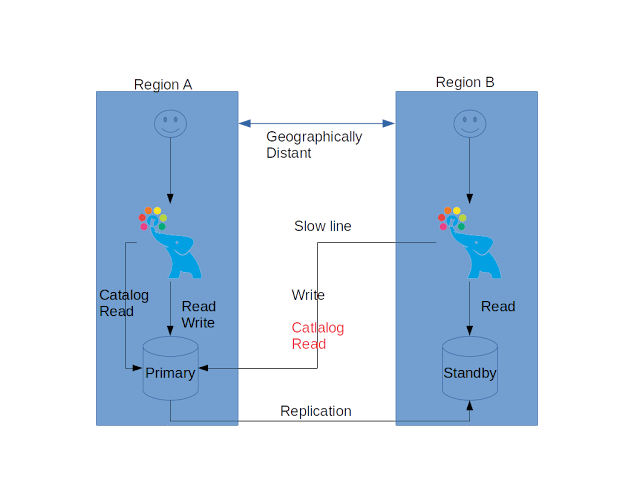
From Pgpool-II 4.1, which is under development, user could eliminate the slow system catalog access in from region B to region A by setting relcache_query_target = load_balance_node and backend weight of primary server to 0 in Pgpool-II running in region B.

Now the system catalog access is redirected to the standby server, rather than to the primary server and the access speed should faster.
Please note that , however, there may be replication delay and that could cause a trouble if the target table is pretty new because the system catalog in the standby server may not the have the new table info. So this configuration is best suitable for a system the table creation is rare, or they are created while users do not access the system.
By the way, Pgpool-II developers define the target date for release 4.1 of Pgpool-II in this October. Please stay tuned.
↧
↧
Pavel Stehule: new releases of plpgsql_check and pspg
Here are plpgsql_check and pspg.
I fixed few significant errors in profiler integrated to plpgsql_check. I hope, so profiler should to work well now.
The bugs fixed in pspg are minor bugfixes.
I fixed few significant errors in profiler integrated to plpgsql_check. I hope, so profiler should to work well now.
The bugs fixed in pspg are minor bugfixes.
↧
Mark Wong: PostgreSQL Award
PostgreSQL was presented with the 2019 O’Reilly Open Source Award for Lifetime Achievement in Portland, Oregon, Thursday July 18th during OSCON. I had the honor of accepting that award alongside Bruce Momjian and Christophe Pettus. Starting last year in 2018, these awards were presented to projects and the first Lifetime Achievement award was given to […]
↧
Devrim GÜNDÜZ: Installing PostgreSQL on RHEL 8
RHEL 8 was released 2 months ago, and we already released RPMs for many of the packages. RHEL 8 support is limited, though -- we will release more packages when EPEL 8 is out.
Because of the modularity feature in RHEL 8, installing PGDG RPMs on RHEL 8 requires extra step. Continue reading "Installing PostgreSQL on RHEL 8 "
Because of the modularity feature in RHEL 8, installing PGDG RPMs on RHEL 8 requires extra step. Continue reading "Installing PostgreSQL on RHEL 8 "
↧