Vacuuming is a key feature of PostgreSQL databases to keep databases healthy and optimized. For this, Autovacuum is configured to conserve space by removing obsolete disk usage, and to optimize database performance by speeding up sequential scans, just as one example. To discuss this topic in-depth, 2ndQuadrant hosted the “Postgres Vacuuming Through Pictures” webinar. The […]
↧
Liaqat Andrabi: Webinar: Postgres Vacuuming Through Pictures [Follow up]
↧
Johann Oskarsson: Running Pgbadger Automatically with Zsh
Here I present a simple script that queries the database for the log file locations and automatically chooses the one for yesterday. The trick here is to apply strftime to the log filename as configured in the database. This way, it doesn’t matter how complex the log file name is in the database, it’s alawys easy to guess. All this works as long as the system’s strftime and PostgreSQL’s log file escapes are equivalent; this should never be an issue.
There are some limits to the current script. It assumes log_directory is to be found within data_directory and is not an absolute path. It also assumes there are no strftime escape sequences in the directory names themselves. Fixing either or both of these is not hard if a more general script is needed. It is also hardcoded to choose the csv log file, but this is easy to change.
Finally it runs pgbadger on the log file from yesterday, and outputs html in the webserver’s directory. The assumption here is that PostgreSQL will write its log into a new file every day, possibly in a rotating sequence.
The script is mean to be called every day with cron.
#!/usr/local/bin/zsh

zmodload zsh/datetime

datadir=`/usr/local/bin/psql -A -t -q -w -c "show data_directory" ;`
logdir=`/usr/local/bin/psql -A -t -q -w -c "show log_directory" ;`
filename=`/usr/local/bin/psql -A -t -q -w -c "show log_filename" ;`

strftime -s log $datadir/$logdir/$filename $(( $epochtime[ 1 ] - 24 * 60 * 60 ))

/usr/local/bin/pgbadger -q -I -O /var/www/html/pgbadger/ -o index.html  ${log:r}.csv
↧
↧
Thom Brown: jsquery vs SQL/JSON
SQL/JSON is coming to PostgreSQL 12 and provides a native way to query JSON data (although, to be specific, JSON data stored as a JSONB data type). This also introduces the jsonpath data type which is used for SQL/JSON query expressions. I'll not be going into its usage in detail, or covering performance characteristics (at least not in this post), but I will compare the syntax and functionality with jsquery. Note that this may potentially change prior to final release.
jsquery was introduced as a non-core extension for PostgreSQL 9.4 and higher by Teodor Sigaev, Alexander Korotkov and Oleg Bartunov. Like jsonpath, it also used its own datatype, jsquery.
We have some functions to which we can pass jsonpath expressions to, 2 of which have operators which can be used as shorthand (albeit without additional parameter control, as they exist primarily for indexing purposes):
These will suppress errors where there's a lack of an array element, object field, an unexpected JSON type or numeric errors.
Here are some examples of how jsquery and SQL/JSON differ in practice. (Note that jsquery usage requires installation of the jsquery extension):
We will select all elements from an array which are equal to 1. Note that, here, jsquery returns an array containing 1, whereas jsonpath returns a scalar value of 1.
jsquery
jsonpath
Now we'll check that all elements are greater than 1 and less than 5.
jsquery
jsonpath
And here we have some jsonb data as follows:
We want books by William Shakespeare.
jsquery
jsonpath
You can see that, while they share some characteristics, they are not the same. It's also possible to control whether it uses lax or strict rules which determine whether or not to throw an error if referencing a non-existing object member or a structural issue. "lax" suppresses such errors, "strict" doesn't. These are placed at the beginning of the jsonpath expression.
So we end up with the following syntax for jsonpath:
I've put together some comparisons between jsquery and jsonpath expressions.
Note that, unlike SQL expressions, you can use the equality operator with "null", whereas you would usually have to state IS NULL. This is because it's not directly equivalent.
For more information on the jsonpath and SQL/JSON, see the PostgreSQL documentation:
SQL/JSON Path Expressions
jsonpath Type
jsquery was introduced as a non-core extension for PostgreSQL 9.4 and higher by Teodor Sigaev, Alexander Korotkov and Oleg Bartunov. Like jsonpath, it also used its own datatype, jsquery.
We have some functions to which we can pass jsonpath expressions to, 2 of which have operators which can be used as shorthand (albeit without additional parameter control, as they exist primarily for indexing purposes):
| Function | Operator | Description |
|---|---|---|
jsonb_path_exists | @? | This will return true if it matched something, false if not, or null if it resulted in an operation on a missing value. |
jsonb_path_match | @@ | This does the same thing as jsonb_path_exists, but only first result item is tested. |
jsonb_path_query | None | Returns the JSON data resulting from the jsonpath expression. |
jsonb_path_query_array | None | Same as jsonb_path_query, but puts the result in a JSON array. |
jsonb_path_query_first | None | Same as jsonb_path_query, but only selects the first value. |
These will suppress errors where there's a lack of an array element, object field, an unexpected JSON type or numeric errors.
Here are some examples of how jsquery and SQL/JSON differ in practice. (Note that jsquery usage requires installation of the jsquery extension):
We will select all elements from an array which are equal to 1. Note that, here, jsquery returns an array containing 1, whereas jsonpath returns a scalar value of 1.
jsquery
SELECT '[1,2,3]'::jsonb ~~ '#. ?($ = 1).$'::jsquery;
jsonpath
SELECT jsonb_path_query('[1,2,3]'::jsonb, '$[*] ? (@ == 1)');Now we'll check that all elements are greater than 1 and less than 5.
jsquery
SELECT '[2,3,4]' @@ '#: ($ > 1 and $ < 5)'::jsquery;
jsonpath
SELECT '[2,3,4]' @? '$[*] ? (@ > 1 && @ < 5)';
And here we have some jsonb data as follows:
CREATE TABLE books (data jsonb);

INSERT INTO books (data) VALUES ('[{"author": "Charles Dickens", "book": "A Tale of Two Cities"},
   {"author": "William Shakespeare", "book": "Hamlet"}]');
We want books by William Shakespeare.
jsquery
SELECT data ~~ '#. ? ($.author = "William Shakespeare")' FROM books;
jsonpath
SELECT jsonb_path_query(data,'$[*] ? (@.author == "William Shakespeare")') FROM books;
You can see that, while they share some characteristics, they are not the same. It's also possible to control whether it uses lax or strict rules which determine whether or not to throw an error if referencing a non-existing object member or a structural issue. "lax" suppresses such errors, "strict" doesn't. These are placed at the beginning of the jsonpath expression.
So we end up with the following syntax for jsonpath:
[lax|strict] <path expression> ? <filter expression>
I've put together some comparisons between jsquery and jsonpath expressions.
| - | Achievable using other jsonpath operators. |
| * | No jsonpath equivalent, but usage available at the SQL level. |
| x | No equivalent. |
| jsquery | jsonpath | Description |
|---|---|---|
$ | $ | The whole document |
. | . | Accessor |
* | * | All values at the current level |
| x | ** | All values at all levels |
#N | $[N] | Nth value of an array starting at 0 |
| x | $[start,end] | Slice of an array |
# | - | All array elements |
% | - | All object keys |
| jsquery | jsonpath | Description |
|---|---|---|
| x | + (unary) | Plus operation on a sequence |
| x | - (unary) | Minus operation on sequence |
| x | + (binary) | Addition |
| x | - (binary) | Subtraction |
| x | * | Multiplication |
| x | / | Division |
IS <type> | type() | Checks the type (jsquery) or returns the type name (jsonpath) |
@# | size() | Size (length) of an array |
| x | double() | Numeric value from string |
| x | ceiling() | Nearest integer greater than or equal to value |
| x | floor() | Nearest integer less than or equal to value |
| x | abs() | Absolute value of number |
| x | keyvalue() | Object represented as sequence of key, value and id fields |
| jsquery | jsonpath | Description |
|---|---|---|
= | == | Equality |
< | < | Less than |
<= | <= | Less than or equal to |
> | > | Greater than |
>= | >= | Greater than or equal to |
@> | * | Contains |
<@ | * | Contained by |
IN | - | Search within a list of scalar values |
&& | * | Overlap |
AND | && | Boolean AND |
OR | || | Boolean OR |
NOT | ! | Boolean NOT |
=* | exists | Expression contains 1 or more items |
starts with | Value begins with specified value | |
| x | like_regex | Test string against regex pattern |
| jsquery | jsonpath |
|---|---|
true | true |
false | false |
null | null |
| x | is unknown |
Note that, unlike SQL expressions, you can use the equality operator with "null", whereas you would usually have to state IS NULL. This is because it's not directly equivalent.
jsquery features not present in SQL/JSON.
jsquery supports index hints, but this was necessary as the optimiser has no knowledge of the contents of jsquery strings or statistics related to individual values. So this feature is effectively redundant when it comes to SQL/JSON.Limitations
Only text, numeric and boolean types are supported at present. Datetime is still a work in progress, so these are intended to be supported in JSONB in future.For more information on the jsonpath and SQL/JSON, see the PostgreSQL documentation:
SQL/JSON Path Expressions
jsonpath Type
↧
Paul Ramsey: Waiting for PostGIS 3: Hilbert Geometry Sorting

With the release of PostGIS 3.0, queries that ORDER BY geometry columns will return rows using a Hilbert curve ordering, and do so about twice as fast.
Whuuuut!?!
The history of "ordering by geometry" in PostGIS is mostly pretty bad. Up until version 2.4 (2017), if you did ORDER BY on a geometry column, your rows would be returned using the ordering of the minimum X coordinate value in the geometry.
One of the things users expect of "ordering" is that items that are "close" to each other in the ordered list should also be "close" to each other in the domain of the values. For example, in a set of sales orders ordered by price, rows next to each other have similar prices.
To visualize what geometry ordering looks like, I started with a field of 10,000 random points.

↧
Álvaro Hernández: Benchmarking: Do it with transparency or don't do it at all
Introduction This post is a reply to MongoDB’s “Benchmarking: Do it right or don’t do it at all” post. Which they wrote as a response to the whitepaper “Performance Benchmark: PostgreSQL / MongoDB”, published and sponsored by EnterpriseDB and performed by OnGres. While a long read at close to 50 pages, we encourage you to at least read the executive summary (2 pages) and any other relevant section, to have the right context.
↧
↧
Sebastian Insausti: Big Data with PostgreSQL and Apache Spark

PostgreSQL is well known as the most advanced opensource database, and it helps you to manage your data no matter how big, small or different the dataset is, so you can use it to manage or analyze your big data, and of course, there are several ways to make this possible, e.g Apache Spark. In this blog, we’ll see what Apache Spark is and how we can use it to work with our PostgreSQL database.
For big data analytics, we have two different types of analytics:
- Batch analytics: Based on the data collected over a period of time.
- Real-time (stream) analytics: Based on an immediate data for an instant result.
What is Apache Spark?
Apache Spark is a unified analytics engine for large-scale data processing that can work on both batch and real-time analytics in a faster and easier way.
It provides high-level APIs in Java, Scala, Python and R, and an optimized engine that supports general execution graphs.
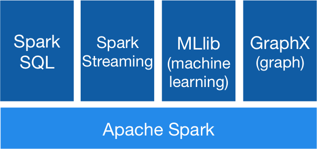
Apache Spark Components
Apache Spark Libraries
Apache Spark includes different libraries:
- Spark SQL: It’s a module for working with structured data using SQL or a DataFrame API. It provides a common way to access a variety of data sources, including Hive, Avro, Parquet, ORC, JSON, and JDBC. You can even join data across these sources.
- Spark Streaming: It makes easy to build scalable fault-tolerant streaming applications using a language-integrated API to stream processing, letting you write streaming jobs the same way you write batch jobs. It supports Java, Scala and Python. Spark Streaming recovers both lost work and operator state out of the box, without any extra code on your part. It lets you reuse the same code for batch processing, join streams against historical data, or run ad-hoc queries on stream state.
- MLib (Machine Learning): It’s a scalable machine learning library. MLlib contains high-quality algorithms that leverage iteration and can yield better results than the one-pass approximations sometimes used on MapReduce.
- GraphX: It’s an API for graphs and graph-parallel computation. GraphX unifies ETL, exploratory analysis, and iterative graph computation within a single system. You can view the same data as both graphs and collections, transform and join graphs with RDDs efficiently, and write custom iterative graph algorithms using the Pregel API.
Apache Spark Advantages
According to the official documentation, some advantages of Apache Spark are:
- Speed: Run workloads 100x faster. Apache Spark achieves high performance for both batch and streaming data, using a state-of-the-art DAG (Direct Acyclic Graph) scheduler, a query optimizer, and a physical execution engine.
- Ease of Use: Write applications quickly in Java, Scala, Python, R, and SQL. Spark offers over 80 high-level operators that make it easy to build parallel apps. You can use it interactively from the Scala, Python, R, and SQL shells.
- Generality: Combine SQL, streaming, and complex analytics. Spark powers a stack of libraries including SQL and DataFrames, MLlib for machine learning, GraphX, and Spark Streaming. You can combine these libraries seamlessly in the same application.
- Runs Everywhere: Spark runs on Hadoop, Apache Mesos, Kubernetes, standalone, or in the cloud. It can access diverse data sources. You can run Spark using its standalone cluster mode, on EC2, on Hadoop YARN, on Mesos, or on Kubernetes. Access data in HDFS, Alluxio, Apache Cassandra, Apache HBase, Apache Hive, and hundreds of other data sources.
Now, let’s see how we can integrate this with our PostgreSQL database.
How to Use Apache Spark with PostgreSQL
We’ll assume you have your PostgreSQL cluster up and running. For this task, we’ll use a PostgreSQL 11 server running on CentOS7.
First, let’s create our testing database on our PostgreSQL server:
postgres=# CREATE DATABASE testing;
CREATE DATABASE
postgres=# \c testing
You are now connected to database "testing" as user "postgres".
Now, we’re going to create a table called t1:
testing=# CREATE TABLE t1 (id int, name text);
CREATE TABLE
And insert some data there:
testing=# INSERT INTO t1 VALUES (1,'name1');
INSERT 0 1
testing=# INSERT INTO t1 VALUES (2,'name2');
INSERT 0 1
Check the data created:
testing=# SELECT * FROM t1;
 id | name
----+-------
  1 | name1
  2 | name2
(2 rows)
To connect Apache Spark to our PostgreSQL database, we’ll use a JDBC connector. You can download it from here.
$ wget https://jdbc.postgresql.org/download/postgresql-42.2.6.jarNow, let’s install Apache Spark. For this, we need to download the spark packages from here.
$ wget http://us.mirrors.quenda.co/apache/spark/spark-2.4.3/spark-2.4.3-bin-hadoop2.7.tgz
$ tar zxvf spark-2.4.3-bin-hadoop2.7.tgz
$ cd spark-2.4.3-bin-hadoop2.7/
To run the Spark shell we’ll need JAVA installed on our server:
$ yum install javaSo now, we can run our Spark Shell:
$ ./bin/spark-shell
Using Spark's default log4j profile: org/apache/spark/log4j-defaults.properties
Setting default log level to "WARN".
To adjust logging level use sc.setLogLevel(newLevel). For SparkR, use setLogLevel(newLevel).
Spark context Web UI available at http://ApacheSpark1:4040
Spark context available as 'sc' (master = local[*], app id = local-1563907528854).
Spark session available as 'spark'.
Welcome to
      ____              __
     / __/__  ___ _____/ /__
    _\ \/ _ \/ _ `/ __/  '_/
   /___/ .__/\_,_/_/ /_/\_\   version 2.4.3
      /_/

Using Scala version 2.11.12 (OpenJDK 64-Bit Server VM, Java 1.8.0_212)
Type in expressions to have them evaluated.
Type :help for more information.

scala>
We can access our Spark context Web UI available in the port 4040 on our server:
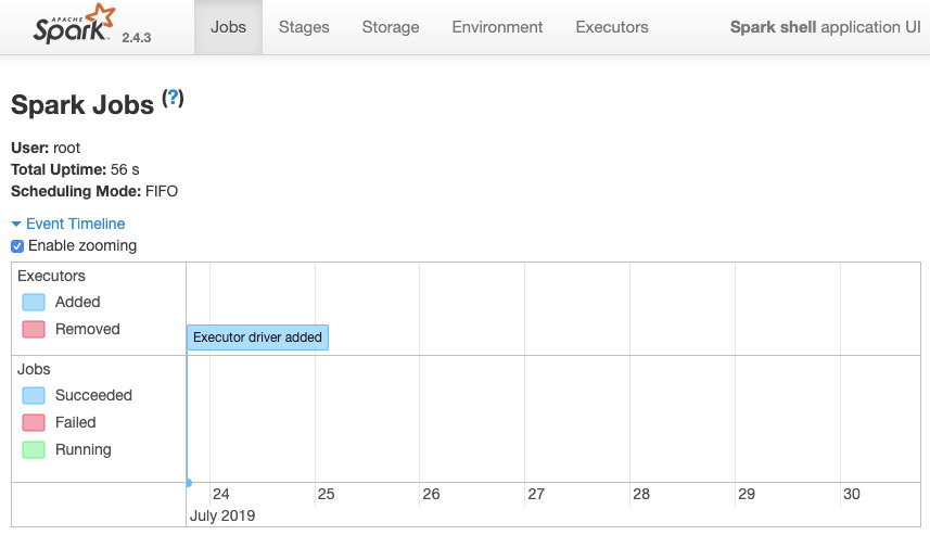
Apache Spark UI
Into the Spark shell, we need to add the PostgreSQL JDBC driver:
scala> :require /path/to/postgresql-42.2.6.jar
Added '/path/to/postgresql-42.2.6.jar' to classpath.
scala> import java.util.Properties
import java.util.Properties
And add the JDBC information to be used by Spark:
scala> val url = "jdbc:postgresql://localhost:5432/testing"
url: String = jdbc:postgresql://localhost:5432/testing
scala> val connectionProperties = new Properties()
connectionProperties: java.util.Properties = {}
scala> connectionProperties.setProperty("Driver", "org.postgresql.Driver")
res6: Object = null
Now, we can execute SQL queries. First, let’s define query1 as SELECT * FROM t1, our testing table.
scala> val query1 = "(SELECT * FROM t1) as q1"
query1: String = (SELECT * FROM t1) as q1
And create the DataFrame:
scala> val query1df = spark.read.jdbc(url, query1, connectionProperties)
query1df: org.apache.spark.sql.DataFrame = [id: int, name: string]
So now, we can perform an action over this DataFrame:
scala> query1df.show()
+---+-----+
| id| name|
+---+-----+
|  1|name1|
|  2|name2|
+---+-----+
scala> query1df.explain
== Physical Plan ==
*(1) Scan JDBCRelation((SELECT * FROM t1) as q1) [numPartitions=1] [id#19,name#20] PushedFilters: [], ReadSchema: struct<id:int,name:string>We can add more values and run it again just to confirm that it’s returning the current values.
PostgreSQL
testing=# INSERT INTO t1 VALUES (10,'name10'), (11,'name11'), (12,'name12'), (13,'name13'), (14,'name14'), (15,'name15');
INSERT 0 6
testing=# SELECT * FROM t1;
 id |  name
----+--------
  1 | name1
  2 | name2
 10 | name10
 11 | name11
 12 | name12
 13 | name13
 14 | name14
 15 | name15
(8 rows)
Spark
scala> query1df.show()
+---+------+
| id|  name|
+---+------+
|  1| name1|
|  2| name2|
| 10|name10|
| 11|name11|
| 12|name12|
| 13|name13|
| 14|name14|
| 15|name15|
+---+------+
In our example, we’re showing only how Apache Spark works with our PostgreSQL database, not how it manages our Big Data information.
Conclusion
Nowadays, it’s pretty common to have the challenge to manage big data in a company, and as we could see, we can use Apache Spark to cope with it and make use of all the features that we mentioned earlier. The big data is a huge world, so you can check the official documentation for more information about the usage of Apache Spark and PostgreSQL and fit it to your requirements.
↧
Michael Paquier: Postgres 12 highlight - Replication slot copy
Replication slots can be used in streaming replication, with physical replication slots, and logical decoding, with logical replication slots, to retain WAL in a more precise way than wal_keep_segments so as past WAL segments are removed at checkpoint using the WAL position a client consuming the slot sees fit. A feature related to replication slots has been committed to PostgreSQL 12:
commit: 9f06d79ef831ffa333f908f6d3debdb654292414
author: Alvaro Herrera <alvherre@alvh.no-ip.org>
date: Fri, 5 Apr 2019 14:52:45 -0300
Add facility to copy replication slots

This allows the user to create duplicates of existing replication slots,
either logical or physical, and even changing properties such as whether
they are temporary or the output plugin used.

There are multiple uses for this, such as initializing multiple replicas
using the slot for one base backup; when doing investigation of logical
replication issues; and to select a different output plugins.

Author: Masahiko Sawada
Reviewed-by: Michael Paquier, Andres Freund, Petr Jelinek
Discussion: https://postgr.es/m/CAD21AoAm7XX8y_tOPP6j4Nzzch12FvA1wPqiO690RCk+uYVstg@mail.gmail.com
This introduces two new SQL functions adapted for each slot type:
- pg_copy_logical_replication_slot
- pg_copy_physical_replication_slot
By default pg_basebackup uses a temporary replication slot to make sure that while transferring the data of the main data folder the WAL segments necessary for recovery from the beginning to the end of the backup are transferred properly, and that the backup does not fail in the middle of processing. In this case the slot is called pg_basebackup_N where N is the PID of the backend process running the replication connection. However there are cases where it makes sense to not use a temporary slot but a permanent one, particularly when reusing a base backup as a standby with no WAL archiving around, so as it is possible to keep WAL around for longer without having a primary’s checkpoint interfere with the recycling of WAL segments. One major take of course with replication slots is that they require a closer monitoring of the local pg_wal/ folder, as if its partition gets full PostgreSQL would immediately stop.
In the case of a physical slot, a copy is useful when creating multiple standbys from the same base backup. As a replication slot can only be consumed by one slot, it reduces the portability of a given base backup, however it is possible to do the following:
- Complete a base backup with pg_basebackup –slot using a permanent slot.
- Create one or more copies of the original slot.
- Use each slot for one standby, which release WAL at their own pace.
Another property of the copy functions is that it is possible to switch a physical slot from temporary to permanent and vice-versa. Here is for example how to create a slot from a permanent one (controlled by the third argument of the function) which retains WAL immediately (controlled by the second argument). The copy of the slot will mark the restart_lsn of the origin slot to be the same as the target:
=# SELECT * FROM pg_create_physical_replication_slot('physical_slot_1', true, false);
    slot_name    |    lsn
-----------------+-----------
 physical_slot_1 | 0/15F2A58
(1 row)
=# select * FROM pg_copy_physical_replication_slot('physical_slot_1', 'physical_slot_2');
    slot_name    | lsn
-----------------+------
 physical_slot_2 | null
(1 row)
=# SELECT slot_name, restart_lsn FROM pg_replication_slots;
    slot_name    | restart_lsn
-----------------+-------------
 physical_slot_1 | 0/15CF098
 physical_slot_2 | 0/15CF098
(2 rows)
Note that it is not possible to copy a physical slot to become a logical one, but that a slot can become temporary after being copied from a permanent one, and that the copied temporary slot will be associated to the session doing the copy:
=# SELECT pg_copy_logical_replication_slot('physical_slot_1', 'logical_slot_2');
ERROR:  0A000: cannot copy logical replication slot "physical_slot_1" as a physical replication slot
LOCATION:  copy_replication_slot, slotfuncs.c:673
=# SELECT * FROM pg_copy_physical_replication_slot('physical_slot_1', 'physical_slot_temp', true);
     slot_name      | lsn
--------------------+------
 physical_slot_temp | null
(1 row)
=# SELECT slot_name, temporary, restart_lsn FROM pg_replication_slots;
     slot_name      | temporary | restart_lsn
--------------------+-----------+-------------
 physical_slot_1    | f         | 0/15CF098
 physical_slot_2    | f         | 0/15CF098
 physical_slot_temp | t         | 0/15CF098
(3 rows)
The copy of logical slots also has many usages. As logical replication makes use of a slot on the publication side which is then consumed by a subscription, this makes the debugging of such configurations easier, particularly if there is a conflict of some kind on the target server. The most interesting property is that it is possible to change two properties of a slot when copying it:
- Change a slot from being permanent or temporary.
- More importantly, change the output plugin of a slot.
In the context of logical replication, the output plugin being used is pgoutput, and here is how to copy a logical slot with a new, different plugin. At creation the third argument controls if a slot is temporary or not:
=# SELECT * FROM pg_create_logical_replication_slot('logical_slot_1', 'pgoutput', false);
   slot_name    |    lsn
----------------+-----------
 logical_slot_1 | 0/15CF7C0
(1 row)
=# SELECT * FROM pg_copy_logical_replication_slot('logical_slot_1', 'logical_slot_2', false, 'test_decoding');
   slot_name    |    lsn
----------------+-----------
 logical_slot_2 | 0/15CF7C0
(1 row)
=# SELECT slot_name, restart_lsn, plugin FROM pg_replication_slots
     WHERE slot_type = 'logical';
   slot_name    | restart_lsn |    plugin
----------------+-------------+---------------
 logical_slot_1 | 0/15CF788   | pgoutput
 logical_slot_2 | 0/15CF788   | test_decoding
(2 rows)
And then the secondary slot can be looked at with more understandable data as it prints text records of logical changes happening. This can be consumed with the SQL functions like pg_logical_slot_get_changes as well as a client like pg_recvlogical.
↧
Hans-Juergen Schoenig: Combined indexes vs. separate indexes in PostgreSQL
A “composite index”, also known as “concatenated index”, is an index on multiple columns in a table. Many people are wondering, what is more beneficial: Using separate or using composite indexes? Whenever we do training, consulting or support this question is high up on the agenda and many people keep asking this question. Therefore, I decided to shed some light on this question.
Which indexes shall one create?
To discuss the topic on a more practical level, I created a table consisting of three columns. Then I loaded 1 million rows and added a composite index covering all three columns:
test=# CREATE TABLE t_data (a int, b int, c int);
CREATE TABLE
test=# INSERT INTO t_data
		SELECT random()*100000,
			random()*100000,
			random()*100000
		FROM generate_series(1, 1000000);
INSERT 0 1000000
test=# CREATE INDEX idx_data ON t_data(a, b, c);
CREATE INDEX
The layout of the table is therefore as follows:
test=# \d t_data
               Table "public.t_data"
 Column |  Type   | Collation | Nullable | Default
--------+---------+-----------+----------+---------
 a      | integer |           |          |
 b      | integer |           |          |
 c      | integer |           |          |
Indexes:
    "idx_data" btree (a, b, c)
Let us run ANALYZE now to ensure that optimizer statistics are there. Usually autovacuum will kick in and create statistics for your table, but to make sure running ANALYZE does not hurt in this case.
test=#  ANALYZE t_data;
ANALYZE
PostgreSQL will rearrange filters for you
The first important thing to observe is that PostgreSQL will try to arrange the filters in your query for you. The following query will filter on all indexed columns:
test=# explain SELECT *
       FROM   t_data
       WHERE  c = 10
              AND b = 20
              AND a = 10;
                   QUERY PLAN
---------------------------------------------------
 Index Only Scan using idx_data on t_data
       (cost=0.42..4.45 rows=1 width=12)
   Index Cond: ((a = 10) AND (b = 20) AND (c = 10))
(2 rows)
As you can see we filtered for c, b, a but the optimizer changed the order of those conditions and turned it into a, b, c to make sure that the index we created suits the query. There are some important things to learn here:
- The order of the conditions in your WHERE clause makes no difference
- PostgreSQL will find the right indexes automatically
Also, keep in mind that PostgreSQL knows that equality is transitive and can infer conditions from that:
test=# explain SELECT *
       FROM    t_data
       WHERE   c = 10
               AND b = a
               AND a = c;
                     QUERY PLAN
---------------------------------------------------
 Index Only Scan using idx_data on t_data
       (cost=0.42..4.45 rows=1 width=12)
   Index Cond: ((a = 10) AND (b = 10) AND (c = 10))
(2 rows)
What you can see here is that PostgreSQL figured out automatically that a, b and c are actually the same.
Using parts of an index
However, if you have a composite index it is not necessary to filter on all columns. It is also ok to use the first or the first and second field to filter on. Here is an example:
test=# explain SELECT *
       FROM    t_data
       WHERE   a = 10;
                 QUERY PLAN
------------------------------------------
 Index Only Scan using idx_data on t_data
       (cost=0.42..4.62 rows=11 width=12)
   Index Cond: (a = 10)
(2 rows)
As you can see PostgreSQL can still use the same index. An index is simple a sorted list, which happens to be ordered by three fields. In multi-column indexes, this ordering is a so-called &ldauo;lexicographical ordering”: the rows are first sorted by the first index column. Rows with the same first column are sorted by the second column, and so on. It is perfectly fine to just make use of the first columns. Talking about sorted lists:
test=# explain SELECT *
       FROM    t_data
       WHERE   a = 10
       ORDER BY b, c;
                QUERY PLAN
-------------------------------------------
 Index Only Scan using idx_data on t_data
       (cost=0.42..4.62 rows=11 width=12)
   Index Cond: (a = 10)
(2 rows)
An index can also provide you with sorted data. In this case we filter on a and order by the remaining two columns b and c.
When composite indexes don’t work
Let us try to understand, when a composite index does not help to speed up a query. Here is an example:
test=# explain SELECT *
       FROM    t_data
       WHERE   b = 10;
                     QUERY PLAN
---------------------------------------------------
 Gather  (cost=1000.00..11615.43 rows=11 width=12)
   Workers Planned: 2
   ->  Parallel Seq Scan on t_data
         (cost=0.00..10614.33 rows=5 width=12)
         Filter: (b = 10)
(4 rows)
In this case we are filtering on the second column. Remember: A btree index is nothing more than a sorted list. In our case it is sorted by a, b, c. So naturally we cannot usefully filter on this field. However, in some rare cases it can happen that you will still see an index scan. Some people see that as proof “that it does indeed work”. But, you will see an index scan for the wrong reason: PostgreSQL is able to read an index completely – not to filter but to reduce the amount of I/O it takes to read a table. If a table has many columns it might be faster to read the index than to digest the table.
Let us simulate this:
test=# SET seq_page_cost TO 10000;
SET
By telling PostgreSQL that sequential I/O is more expensive than it really is you will see that the optimizer turns to an index scan:
test=# explain analyze
       SELECT *
       FROM   t_data
       WHERE  b = 10;
                  QUERY PLAN
--------------------------------------------------
 Index Only Scan using idx_data on t_data
       (cost=0.42..22892.53 rows=11 width=12)
       (actual time=7.626..63.087 rows=8 loops=1)
   Index Cond: (b = 10)
   Heap Fetches: 0
 Planning Time: 0.121 ms
 Execution Time: 63.122 ms
(5 rows)
However, the execution time is 63 milliseconds, which is A LOT more than if we had done this for the first column in the index.
Note that “Index Cond: (b = 10)” means something different here than in the previous examples: while before we had index scan conditions, here we have an index filter condition. It is not ideal that the two look the same in the EXPLAIN output.
Understanding bitmap index scans in PostgreSQL
PostgreSQL is able to use more than one index at the same time. This is especially important if you are using OR as shown in the next example:
test=# SET seq_page_cost TO default;
SET
test=# explain SELECT *
       FROM    t_data
       WHERE   a = 4
               OR a = 23232;
                     QUERY PLAN
----------------------------------------------------
 Bitmap Heap Scan on t_data
        (cost=9.03..93.15 rows=22 width=12)
   Recheck Cond: ((a = 4) OR (a = 23232))
   ->  BitmapOr  (cost=9.03..9.03 rows=22 width=0)
         ->  Bitmap Index Scan on idx_data
               (cost=0.00..4.51 rows=11 width=0)
               Index Cond: (a = 4)
         ->  Bitmap Index Scan on idx_data
               (cost=0.00..4.51 rows=11 width=0)
               Index Cond: (a = 23232)
(7 rows)
What PostgreSQL will do is to decide on a bitmap scan. The idea is to first consult all the indexes to compile a list of rows / blocks, which then have to be fetched from the table (= heap). This is usually a lot better than a sequential scan. In my example the same index is even used twice. However, in real life you might see bitmap scans involving various indexes more often.
Using a subset of indexes in a single SQL statement
In many cases using too many indexes can even be counterproductive. The planner will make sure that enough indexes are chosen but it won’t take too many. Let us take a look at the following example:
test=# DROP INDEX idx_data;
DROP INDEX
test=# CREATE INDEX idx_a ON t_data (a);
CREATE INDEX
test=# CREATE INDEX idx_a ON t_data (b);
CREATE INDEX
test=# CREATE INDEX idx_a ON t_data (c);
CREATE INDEX
test=# \d t_data
               Table "public.t_data"
 Column |  Type   | Collation | Nullable | Default
--------+---------+-----------+----------+---------
 a      | integer |           |          |
 b      | integer |           |          |
 c      | integer |           |          |
Indexes:
    "idx_a" btree (a)
    "idx_b" btree (b)
    "idx_c" btree (c)
The following query filters on all columns again. This time I did not use a single combined index but decided on separate indexes, which is usually more inefficient. Here is what happens:
test=# explain SELECT *
       FROM    t_data
       WHERE   a = 10
               AND b = 20
               AND c = 30;
                     QUERY PLAN
----------------------------------------------------
 Bitmap Heap Scan on t_data
        (cost=9.27..13.28 rows=1 width=12)
   Recheck Cond: ((c = 30) AND (b = 20))
   Filter: (a = 10)
   ->  BitmapAnd  (cost=9.27..9.27 rows=1 width=0)
         ->  Bitmap Index Scan on idx_c
               (cost=0.00..4.51 rows=11 width=0)
               Index Cond: (c = 30)
         ->  Bitmap Index Scan on idx_b
               (cost=0.00..4.51 rows=11 width=0)
               Index Cond: (b = 20)
(8 rows)
Let us take a closer look at the plan. The query filters on 3 columns BUT PostgreSQL only decided on two indexes. Why is that the case? We have imported 1 million rows. Each column contains 100.000 distinct values, which means that every value occurs 10 times. What is the point in fetching a couple of rows from every index even if two indexes already narrow down the result sufficiently enough? This is exactly what happens.
Optimizing min / max in SQL queries
Indexes are not only about filtering. It will also help you to mind the lowest and the highest value in a column as shown by the following SQL statement:
test=# explain SELECT min(a), max(b) FROM t_data;
                               QUERY PLAN
-----------------------------------------------------------------------
 Result  (cost=0.91..0.92 rows=1 width=8)
   InitPlan 1 (returns $0)
     ->  Limit  (cost=0.42..0.45 rows=1 width=4)
           ->  Index Only Scan using idx_a on t_data
               (cost=0.42..28496.42 rows=1000000 width=4)
                 Index Cond: (a IS NOT NULL)
   InitPlan 2 (returns $1)
     ->  Limit  (cost=0.42..0.45 rows=1 width=4)
           ->  Index Only Scan Backward using idx_b on t_data t_data_1
                 (cost=0.42..28496.42 rows=1000000 width=4)
                 Index Cond: (b IS NOT NULL)
(9 rows)
As you can see PostgreSQL is already pretty sophisticated. If you are looking for good performance it certainly makes sense to see, how PostgreSQL handles indexes and review your code in order to speed thing up. If you want to learn more about performance, consider checking out Laurenzs Albe’s post about speeding up count(*). Also, if you are not sure, why your database is slow, check out my post on PostgreSQL database performance, which explains, how to find slow queries.
The post Combined indexes vs. separate indexes in PostgreSQL appeared first on Cybertec.
↧
Paul Ramsey: PostGIS Overlays
One question that comes up often during our PostGIS training is “how do I do an overlay?” The terminology can vary: sometimes they call the operation a “union” sometimes an “intersect”. What they mean is, “can you turn a collection of overlapping polygons into a collection of non-overlapping polygons that retain information about the overlapping polygons that formed them?”

So an overlapping set of three circles becomes a non-overlapping set of 7 polygons.

Calculating the overlapping parts of a pair of shapes is easy, using the ST_Intersection() function in PostGIS, but that only works for pairs, and doesn’t capture the areas that have no overlaps at all.
How can we handle multiple overlaps and get out a polygon set that covers 100% of the area of the input sets? By taking the polygon geometry apart into lines, and then building new polygons back up.
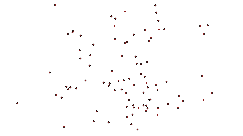
Let’s construct a synthetic example: first, generate a collection of random points, using a Gaussian distribution, so there’s more overlap in the middle. The crazy math in the SQL below just converts the uniform random numbers from the random() function into normally distributed numbers.
CREATETABLEptsASWITHrandsAS(SELECTgenerate_seriesasid,random()ASu1,random()ASu2FROMgenerate_series(1,100))SELECTid,ST_SetSRID(ST_MakePoint(50*sqrt(-2*ln(u1))*cos(2*pi()*u2),50*sqrt(-2*ln(u1))*sin(2*pi()*u2)),4326)ASgeomFROMrands;The result looks like this:
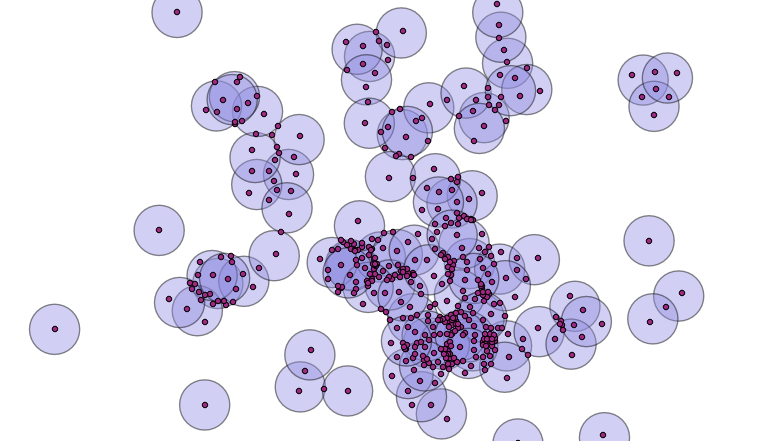
Now, we turn the points into circles, big enough to have overlaps.
CREATETABLEcirclesASSELECTid,ST_Buffer(geom,10)ASgeomFROMpts;Which looks like this:

Now it’s time to take the polygons apart. In this case we’ll take the exterior ring of the circles, using ST_ExteriorRing(). If we were dealing with complex polygons with holes, we’d have to use ST_DumpRings(). Once we have the rings, we want to make sure that everywhere rings cross the lines are broken, so that no lines cross, they only touch at their end points. We do that with the ST_Union() function.
CREATETABLEboundariesASSELECTST_Union(ST_ExteriorRing(geom))ASgeomFROMcircles;What comes out is just lines, but with end points at every crossing.

Now that we have noded lines, we can collect them into a multi-linestring and feed them to ST_Polygonize() to generate polygons. The polygons come out as one big multi-polygon, so we’ll use ST_Dump() to convert it into a table with one row per polygon.
CREATESEQUENCEpolyseq;CREATETABLEpolysASSELECTnextval('polyseq')ASid,(ST_Dump(ST_Polygonize(geom))).geomASgeomFROMboundaries;Now we have a set of polygons with no overlaps, only one polygon per area.

So, how do we figure out how many overlaps contributed to each incoming polygon? We can join the centroids of the new small polygons with the set of original circles, and calculate how many circles contain each centroid point.
A spatial join will allow us to calculate the number of overlaps.
ALTERTABLEpolysADDCOLUMNcountINTEGERDEFAULT0;UPDATEPOLYSsetcount=p.countFROM(SELECTcount(*)AScount,p.idASidFROMpolyspJOINcirclescONST_Contains(c.geom,ST_PointOnSurface(p.geom))GROUPBYp.id)ASpWHEREp.id=polys.id;That’s it! Now we have a single coverage of the area, where each polygon knows how much overlap contributed to it. Ironically, when visualized using the coverage count as a variable in the color ramp, it looks a lot like the original image, which was created with a simple transparency effect. However, the point here is that we’ve created new data, in the count attribute of the new polygon layer.

The same decompose-and-rebuild-and-join-centroids trick can be used to overlay all kinds of features, and to carry over attributes from the original input data, achieving the classic “GIS overlay” workflow. Happy geometry mashing!
↧
↧
Ibrar Ahmed: Parallelism in PostgreSQL

 PostgreSQL is one of the finest object-relational databases, and its architecture is process-based instead of thread-based. While almost all the current database systems utilize threads for parallelism, PostgreSQL’s process-based architecture was implemented prior to POSIX threads. PostgreSQL launches a process “postmaster” on startup, and after that spans new process whenever a new client connects to the PostgreSQL.
Before version 10 there was no parallelism in a single connection. It is true that multiple queries from the different clients can have parallelism because of process architecture, but they couldn’t gain any performance benefit from one another. In other words, a single query runs serially and did not have parallelism. This is a huge limitation because a single query cannot utilize the multi-core. Parallelism in PostgreSQL was introduced from version 9.6. Parallelism, in a sense, is where a single process can have multiple threads to query the system and utilize the multicore in a system. This gives PostgreSQL intra-query parallelism.
Parallelism in PostgreSQL was implemented as part of multiple features which cover sequential scans, aggregates, and joins.
Components of Parallelism in PostgreSQL
There are three important components of parallelism in PostgreSQL. These are the process itself, gather, and workers. Without parallelism the process itself handles all the data, however, when planner decides that a query or part of it can be parallelized, it adds a Gather node within the parallelizable portion of the plan and makes a gather root node of that subtree. Query execution starts at the process (leader) level and all the serial parts of the plan are run by the leader. However, if parallelism is enabled and permissible for any part (or whole) of the query, then gather node with a set of workers is allocated for it. Workers are the threads that run in parallel with part of the tree (partial-plan) that needs to be parallelized. The relation’s blocks are divided amongst threads such that the relation remains sequential. The number of threads is governed by settings as set in PostgreSQL’s configuration file. The workers coordinate/communicate using shared memory, and once workers have completed their work, the results are passed on to the leader for accumulation.

Parallel Sequential Scans
In PostgreSQL 9.6, support for the parallel sequential scan was added. A sequential scan is a scan on a table in which a sequence of blocks is evaluated one after the other. This, by its very nature, allows parallelism. So this was a natural candidate for the first implementation of parallelism. In this, the whole table is sequentially scanned in multiple worker threads. Here is the simple query where we query the pgbench_accounts table rows (63165) which has 1500000000 tuples. The total execution time is 4343080ms. As there is no index defined, the sequential scan is used. The whole table is scanned in a single process with no thread. Therefore the single core of CPU is used regardless of how many cores are available.
db=# EXPLAIN ANALYZE SELECT *
            FROM pgbench_accounts
            WHERE abalance > 0;
                             QUERY PLAN
----------------------------------------------------------------------
 Seq Scan on pgbench_accounts (cost=0.00..73708261.04 rows=1 width=97)
                (actual time=6868.238..4343052.233 rows=63165 loops=1)
   Filter: (abalance > 0)
   Rows Removed by Filter: 1499936835
 Planning Time: 1.155 ms
 Execution Time: 4343080.557 ms
(5 rows)
What if these 1,500,000,000 rows scanned parallel using “10” workers within a process? It will reduce the execution time drastically.
db=# EXPLAIN ANALYZE select * from pgbench_accounts where abalance > 0;
                             QUERY PLAN
----------------------------------------------------------------------
Gather  (cost=1000.00..45010087.20 rows=1 width=97)
        (actual time=14356.160..1628287.828 rows=63165 loops=1)
   Workers Planned: 10
   Workers Launched: 10
   ->  Parallel Seq Scan on pgbench_accounts
              (cost=0.00..45009087.10 rows=1 width=97)
              (actual time=43694.076..1628068.096 rows=5742 loops=11)
   Filter: (abalance > 0)
   Rows Removed by Filter: 136357894
Planning Time: 37.714 ms
Execution Time: 1628295.442 ms
(8 rows)
Now the total execution time is 1628295ms; this is a 266% improvement while using 10 workers thread used to scan.
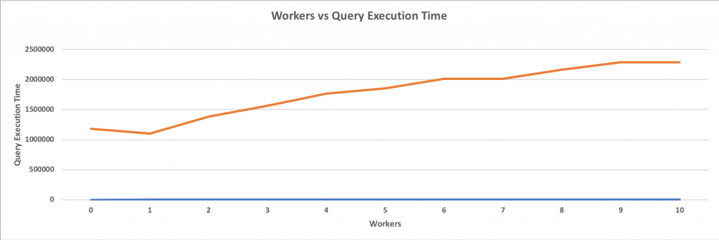
Query used for the Benchmark: SELECT * FROM pgbench_accounts WHERE abalance > 0;
Size of Table: 426GB
Total Rows in Table: 1500000000
The system used for the Benchmark:
CPU: 2 Intel(R) Xeon(R) CPU E5-2643 v2 @ 3.50GHz
RAM: 256GB DDR3 1600
DISK: ST3000NM0033
The above graph clearly shows how parallelism improves performance for a sequential scan. When a single worker is added, the performance understandably degrades as no parallelism is gained, but the creation of an additional gather node and a single work adds overhead. However, with more than one worker thread, the performance improves significantly. Also, it is important to note that performance doesn’t increase in a linear or exponential fashion. It improves gradually until the addition of more workers will not give any performance boost; sort of like approaching a horizontal asymptote. This benchmark was performed on a 64-core machine, and it is clear that having more than 10 workers will not give any significant performance boost.
Parallel Aggregates
In databases, calculating aggregates are very expensive operations. When evaluated in a single process, these take a reasonably long time. In PostgreSQL 9.6, the ability to calculate these in parallel was added by simply dividing these in chunks (a divide and conquer strategy). This allowed multiple workers to calculate the part of aggregate before the final value(s) based on these calculations was calculated by the leader. More technically speaking, PartialAggregate nodes are added to a plan tree, and each PartialAggregate node takes the output from one worker. These outputs are then emitted to a FinalizeAggregate node that combines the aggregates from multiple (all) PartialAggregate nodes. So effectively, the parallel partial plan includes a FinalizeAggregate node at the root and a Gather node which will have PartialAggregate nodes as children.

db=# EXPLAIN ANALYZE SELECT count(*) from pgbench_accounts;
                               QUERY PLAN
----------------------------------------------------------------------
 Aggregate  (cost=73708261.04..73708261.05 rows=1 width=8)
            (actual time=2025408.357..2025408.358 rows=1 loops=1)
   ->  Seq Scan on pgbench_accounts  (cost=0.00..67330666.83 rows=2551037683 width=0)
                                     (actual time=8.162..1963979.618 rows=1500000000 loops=1)
 Planning Time: 54.295 ms
 Execution Time: 2025419.744 ms
(4 rows)
Following is an example of a plan when an aggregate is to be evaluated in parallel. You can clearly see performance improvement here.
db=# EXPLAIN ANALYZE SELECT count(*) from pgbench_accounts;
                           QUERY PLAN
----------------------------------------------------------------------
Finalize Aggregate  (cost=45010088.14..45010088.15 rows=1 width=8)
                 (actual time=1737802.625..1737802.625 rows=1 loops=1)
   ->  Gather  (cost=45010087.10..45010088.11 rows=10 width=8)
               (actual time=1737791.426..1737808.572 rows=11 loops=1)
         Workers Planned: 10
         Workers Launched: 10
         ->  Partial Aggregate
             (cost=45009087.10..45009087.11 rows=1 width=8)
             (actual time=1737752.333..1737752.334 rows=1 loops=11)
             ->  Parallel Seq Scan on pgbench_accounts
                (cost=0.00..44371327.68 rows=255103768 width=0)
              (actual time=7.037..1731083.005 rows=136363636 loops=11)
 Planning Time: 46.031 ms
 Execution Time: 1737817.346 ms
(8 rows)
With parallel aggregates, in this particular case, we get a performance boost of just over 16% as the execution time of 2025419.744 is reduced to 1737817.346 when 10 parallel workers are involved.
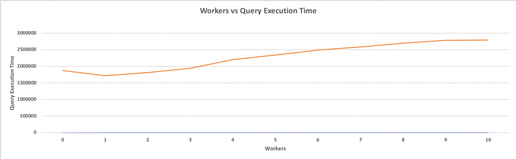
Query used for the Benchmark: SELECT count(*) FROM pgbench_accounts WHERE abalance > 0;
Size of Table: 426GB
Total Rows in Table: 1500000000
The system used for the Benchmark:
CPU: 2 Intel(R) Xeon(R) CPU E5-2643 v2 @ 3.50GHz
RAM: 256GB DDR3 1600
DISK: ST3000NM0033
Parallel Index (B-Tree) Scans
The parallel support for B-Tree index means index pages are scanned in parallel. The B-Tree index is one of the most used indexes in PostgreSQL. In a parallel version of B-Tree, a worker scans the B-Tree and when it reaches its leaf node, it then scans the block and triggers the blocked waiting worker to scan the next block.
Confused? Let’s look at an example of this. Suppose we have a table foo with id and name columns, with 18 rows of data. We create an index on the id column of table foo. A system column CTID is attached with each row of table which identifies the physical location of the row. There are two values in the CTID column: the block number and the offset.
postgres=# SELECT ctid, id FROM foo;
  ctid  | id
--------+-----
 (0,55) | 200
 (0,56) | 300
 (0,57) | 210
 (0,58) | 220
 (0,59) | 230
 (0,60) | 203
 (0,61) | 204
 (0,62) | 300
 (0,63) | 301
 (0,64) | 302
 (0,65) | 301
 (0,66) | 302
 (1,31) | 100
 (1,32) | 101
 (1,33) | 102
 (1,34) | 103
 (1,35) | 104
 (1,36) | 105
(18 rows)
Let’s create the B-Tree index on that table’s id column.
CREATE INDEX foo_idx ON foo(id)

Suppose we want to select values where id <= 200 with 2 workers. Worker-0 will start from the root node and scan until the leaf node 200. It’ll handover the next block under node 105 to Worker-1, which is in a blocked and wait-state. If there are other workers, blocks are divided into the workers. A similar pattern is repeated until the scan is completed.
Parallel Bitmap Scans
To parallelize a bitmap heap scan, we need to be able to divide blocks among workers in a way very similar to parallel sequential scan. To do that, a scan on one or more indexes is done and a bitmap indicating which blocks are to be visited is created. This is done by a leader process, i.e. this part of the scan is run sequentially. However, the parallelism kicks in when the identified blocks are passed to workers, the same way as in a parallel sequential scan.
Parallel Joins
Parallelism in the merge joins support is also one of the hottest features added in this release. In this, a table joins with other tables’ inner loop hash or merge. In any case, there is no parallelism supported in the inner loop. The entire loop is scanned as a whole, and the parallelism occurs when each worker executes the inner loop as a whole. The results of each join sent to gather accumulate and produce the final results.

Summary
It is obvious from what we’ve already discussed in this blog that parallelism gives significant performance boosts for some, slight gains for others, and may cause performance degradation in some cases. Ensure that parallel_setup_cost or parallel_tuple_cost are set up correctly to enable the query planner to choose a parallel plan. Even after setting low values for these GUIs, if a parallel plan is not produced, refer to the PostgreSQL documentation on parallelism for details.
For a parallel plan, you can get per-worker statistics for each plan node to understand how the load is distributed amongst workers. You can do that through EXPLAIN (ANALYZE, VERBOSE). As with any other performance feature, there is no one rule that applies to all workloads. Parallelism should be carefully configured for whatever the need may be, and you must ensure that the probability of gaining performance is significantly higher than the probability of a drop in performance.
↧
Viorel Tabara: Cloud Vendor Deep-Dive: PostgreSQL on AWS Aurora

How deep should we go with this? I’ll start by saying that as of this writing, I could locate only 3 books on Amazon about PostgreSQL in the cloud, and 117 discussions on PostgreSQL mailing lists about Aurora PostgreSQL. That doesn’t look like a lot, and it leaves me, the curious PostgreSQL end user, with the official documentation as the only place where I could really learn some more. As I don’t have the ability, nor the knowledge to adventure myself much deeper, there is AWS re:Invent 2018 for those who are looking for that kind of thrill. I can settle for Werner’s article on quorums.
To get warmed up, I started from the Aurora PostgreSQL homepage where I noted that the benchmark showing that Aurora PostgreSQL is three times faster than a standard PostgreSQL running on the same hardware dates back to PostgreSQL 9.6. As I’ve learned later, 9.6.9 is currently the default option when setting up a new cluster. That is very good news for those who don’t want to, or cannot upgrade right away. And why only 99.99% availability? One explanation can be found in Bruce Momjian’s article.
Compatibility
According to AWS, Aurora PostgreSQL is a drop-in replacement for PostgreSQL, and the documentation states:
The code, tools, and applications you use today with your existing MySQL and PostgreSQL databases can be used with Aurora.
That is reinforced by Aurora FAQs:
It means that most of the code, applications, drivers and tools you already use today with your PostgreSQL databases can be used with Aurora with little or no change. The Amazon Aurora database engine is designed to be wire-compatible with PostgreSQL 9.6 and 10, and supports the same set of PostgreSQL extensions that are supported with RDS for PostgreSQL 9.6 and 10, making it easy to move applications between the two engines.
“most” in the above text suggests that there isn’t a 100% guarantee in which case those seeking certainty should consider purchasing technical support from either AWS Professional Services, or Aamazon Aurora partners. As a side note, I did notice that none of the PostgreSQL professional Hosting Providers employing core community contributors are on that list.
From Aurora FAQs page we also learn that Aurora PostgreSQL supports the same extensions as RDS, which in turn lists most of the community extensions and a few extras.
Concepts
As part of Amazon RDS, Aurora PostgreSQL comes with its own terminology:
- Cluster: A Primary DB instance in read/write mode and zero or more Aurora Replicas. The primary DB is often labeled a Master in `AWS diagrams`_, or Writer in the AWS Console. Based on the reference diagram we can make an interesting observation: Aurora writes three times. As the latency between the AZs is typically higher than within the same AZ, the transaction is considered committed as soon it's written on the data copy within the same AZ, otherwise the latency and potential outages between AZs.
- Cluster Volume: Virtual database storage volume spanning multiple AZs.
- Aurora URL: A `host:port` pair.
- Cluster Endpoint: Aurora URL for the Primary DB. There is one Cluster Endpoint.
- Reader Endpoint: Aurora URL for the replica set. To make an analogy with DNS it's an alias (CNAME). Read requests are load balanced between available replicas.
- Custom Endpoint: Aurora URL to a group consisting of one or more DB instances.
- Instance Endpoint: Aurora URL to a specific DB instance.
- Aurora Version: Product version returned by `SELECT AURORA_VERSION();`.
PostgreSQL Performance and Monitoring on AWS Aurora
Sizing
Aurora PostgreSQL applies a best guess configuration which is based on the DB instance size and storage capacity, leaving further tuning to the DBA through the use of DB Parameters groups.
When selecting the DB instance, base your selection on the desired value for max_connections.
Scaling
Aurora PostgreSQL features auto and manual scaling. Horizontal scaling of read replicas is automated through the use of performance metrics. Vertical scaling can be automated via APIs.
Horizontal scaling takes the offline for a few minutes while replacing compute engine and performing any maintenance operations (upgrades, patching). Therefore AWS recommend performing such operations during maintenance windows.
Scaling in both directions is a breeze:
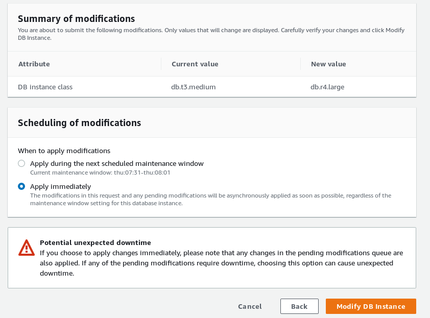
Vertical scaling: modifying instance class

Horizontal scaling: adding reader replica.
At the storage level, space is added in 10G increments. Allocated storage is never reclaimed, see below for how to address this limitation.
Storage
As mentioned above, Aurora PostgreSQL was engineered to take advantage of quorums in order to improve performance consistency.
Since the underlying storage is shared by all DB instances within the same cluster, no additional writes on standby nodes are required. Also, adding or removing DB instances doesn’t change the underlying data.
Wondering what those IOs units mean on the monthly bill? Aurora FAQs comes to the rescue again to explain what an IO is, in the context of monitoring and billing. A Read IO as the equivalent of an 8KiB database page read, and a Write IO as the equivalent of 4KiB written to the storage layer.
High Concurrency
In order to take full advantage of Aurora’s high-concurrency design, it is recommended that applications are configured to drive a large number of concurrent queries and transactions.
Applications designed to direct read and write queries to respectively standby and primary database nodes will benefit from Aurora PostgreSQL reader replica endpoint.
Connections are load balanced between read replicas.
Using custom endpoints database instances with more capacity can be grouped together in order to run an intensive workload such as analytics.
DB Instance Endpoints can be used for fine-grained load balancing or fast failover.
Note that in order for the Reader Endpoints to load balance individual queries, each query must be sent as a new connection.
Caching
Aurora PostgreSQL uses a Survivable Cache Warming technique which ensures that the date in the buffer cache is preserved, eliminating the need for repopulating or warming-up the cache following a database restart.
Replication
Replication lag time between replicas is kept within single digit millisecond. Although not available for PostgreSQL, it’s good to know that cross-region replication lag is kept within 10s of milliseconds.
According to documentation replica lag increases during periods of heavy write requests.
Query Execution Plans
Based on the assumption that query performance degrades over time due to various database changes, the role of this Aurora PostgreSQL component is to maintain a list of approved or rejected query execution plans.
Plans are approved or rejected using either proactive or reactive methods.
When an execution plan is marked as rejected, the Query Execution Plan overrides the PostgreSQL optimizer decisions and prevents the “bad” plan from being executed.
This feature requires Aurora 2.1.0 or later.
PostgreSQL High Availability and Replication on AWS Aurora
At the storage layer, Aurora PostgreSQL ensures durability by replicating each 10GB of storage volume, six times across 3 AZs (each region consists of typically 3 AZs) using physical synchronous replication. That makes it possible for database writes to continue working even when 2 copies of data are lost. Read availability survives the loss of 3 copies of data.
Read replicas ensure that a failed primary instance can be quickly replaced by promoting one of the 15 available replicas. When selecting a multi-AZ deployment one read replica is automatically created. Failover requires no user intervention, and database operations resume in less than 30 seconds.
For single-AZ deployments, the recovery procedure includes a restore from the last known good backup. According to Aurora FAQs the process completes in under 15 minutes if the database needs to be restored in a different AZ. The documentation isn’t that specific, claiming that it takes less than 10 minutes to complete the restore process.
No change is required on the application side in order to connect to the new DB instance as the cluster endpoint doesn’t change during a replica promotion or instance restore.
Step 1: delete the primary instance to force a failover:
Automatic failover Step 1: delete primary
Step 2: automatic failover completed
Automatic failover Step 2: failover completed.
For busy databases, the recovery time following a restart or crash is dramatically reduced since Aurora PostgreSQL doesn’t need to replay the transaction logs.
As part of full-managed service, bad data blocks and disks are automatically replaced.
Failover when replicas exist takes up to 120 seconds with often time under 60 seconds. Faster recovery times can be achieved by when failover conditions are pre-determined, in which case replicas can be assigned failover priorities.
Aurora PostgreSQL plays nice with Amazon RDS – an Aurora instance can act as a read replica for a primary RDS instance.
Aurora PostgreSQL supports Logical Replication which, just like in the community version, can be used to overcome built-in replication limitations. There is no automation or AWS console interface.
Security for PostgreSQL on AWS Aurora
At network level, Aurora PostgreSQL leverages AWS core components, VPC for cloud network isolation and Security Groups for network access control.
There is no superuser access. When creating a cluster, Aurora PostgreSQL creates a master account with a subset of superuser permissions:
postgres@pg107-dbt3medium-restored-cluster:5432 postgres> \du+ postgres
                               List of roles
 Role name |          Attributes               |    Member of       | Description
-----------+-------------------------------+-----------------+-------------
 postgres  | Create role, Create DB           +| {rds_superuser} |
            | Password valid until infinity  |                 |
To secure data in transit, Aurora PostgreSQL provides native SSL/TLS support which can be configured per DB instance.
All data at rest can be encrypted with minimal performance impact. This also applies to backups, snapshots, and replicas.
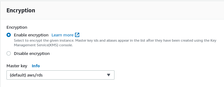
Encryption at rest.
Authentication is controlled by IAM policies, and tagging allows further control over what users are allowed to do and on what resources.
API calls used by all cloud services are logged in CloudTrail.
Client side Restricted Password Management is available via the rds.restrict_password_commands parameter.
PostgreSQL Backup and Recovery on AWS Aurora
Backups are enabled by default and cannot be disabled. They provide point-in-time-recovery using a full daily snapshot as a base backup.
Restoring from an automated backup has a couple of disadvantages: the time to restore may be several hours and data loss may be up to 5 minutes preceding the outage. Amazon RDS Multi-AZ Deployments solve this problem by promoting a read replica to primary, with no data loss.
Database Snapshots are fast and don’t impact the cluster performance. They can be copied or shared with other users.
Taking a snapshot is almost instantaneous:
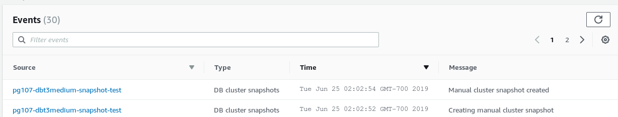
Snapshot time.
Restoring a snapshot is also fast. Compare with PITR:
Backups and snapshots are stored in S3 which offers eleven 9’s of durability.
Aside from backups and snapshots, Aurora PostgreSQL allows databases to be cloned. This is an efficient method for creating copies of large data sets. For example, cloning multi-terabytes of data take only minutes and there is no performance impact.
Aurora PostgreSQL - Point-in-Time Recovery Demo
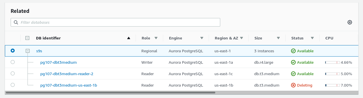
Connecting to cluster:
~ $ export PGUSER=postgres PGPASSWORD=postgres PGHOST=s9s-us-east-1.cluster-ctfirtyhadgr.us-east-1.rds.amazonaws.com
~ $ psql
Pager usage is off.
psql (11.3, server 10.7)
SSL connection (protocol: TLSv1.2, cipher: ECDHE-RSA-AES256-GCM-SHA384, bits: 256, compression: off)
Type "help" for help.
Populate a table with data:
postgres@s9s-us-east-1:5432 postgres> create table s9s (id serial not null, msg text, created timestamptz not null default now());
CREATE TABLE

postgres@s9s-us-east-1:5432 postgres> select * from s9s;
id | msg  |            created
----+------+-------------------------------
1 | test | 2019-06-25 07:57:40.022125+00
2 | test | 2019-06-25 07:57:57.666222+00
3 | test | 2019-06-25 07:58:05.593214+00
4 | test | 2019-06-25 07:58:08.212324+00
5 | test | 2019-06-25 07:58:10.156834+00
6 | test | 2019-06-25 07:59:58.573371+00
7 | test | 2019-06-25 07:59:59.5233+00
8 | test | 2019-06-25 08:00:00.318474+00
9 | test | 2019-06-25 08:00:11.153298+00
10 | test | 2019-06-25 08:00:12.287245+00
(10 rows)
Initiate the restore:
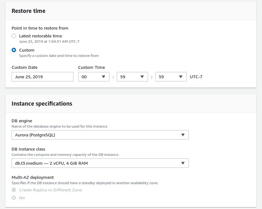
Point-in-Time Recovery: initiate restore.
Once the restore is complete log in and check:
~ $ psql -h pg107-dbt3medium-restored-cluster.cluster-ctfirtyhadgr.us-east-1.rds.amazonaws.com
Pager usage is off.
psql (11.3, server 10.7)
SSL connection (protocol: TLSv1.2, cipher: ECDHE-RSA-AES256-GCM-SHA384, bits: 256, compression: off)
Type "help" for help.

postgres@pg107-dbt3medium-restored-cluster:5432 postgres> select * from s9s;
id | msg  |            created
----+------+-------------------------------
1 | test | 2019-06-25 07:57:40.022125+00
2 | test | 2019-06-25 07:57:57.666222+00
3 | test | 2019-06-25 07:58:05.593214+00
4 | test | 2019-06-25 07:58:08.212324+00
5 | test | 2019-06-25 07:58:10.156834+00
6 | test | 2019-06-25 07:59:58.573371+00
(6 rows)
Best Practices
Monitoring and Auditing
- Integrate database activity streams with third party monitoring in order to monitor database activity for compliance and regulatory requirements.
- A fully-managed database service doesn’t mean lack of responsibility — define metrics to monitor the CPU, RAM, Disk Space, Network, and Database Connections.
- Aurora PostgreSQL integrates with AWS standard monitoring tool CloudWatch, as well as providing additional monitors for Aurora Metrics, Aurora Enhanced Metrics, Performance Insight Counters, Aurora PostgreSQL Replication, and also for RDS Metrics that can be further grouped by RDS Dimensions.
- Monitor Average Active Sessions DB Load by Wait for signs of connections overhead, SQL queries that need tuning, resource contention or an undersized DB instance class.
- Setup Event Notifications.
- Configure error log parameters.
- Monitor configuration changes to database cluster components: instances, subnet groups, snapshots, security groups.
Replication
- Use native table partitioning for workloads that exceed the maximum DB instance class and storage capacity
Encryption
- Encrypted database must have backups enabled to ensure data can be restored in case the encryption key is revoked.
Master Account
- Do not use psql to change the master user password.
Sizing
- Consider using different instance classes in a cluster in order to reduce costs.
Parameter Groups
- Fine tune using Parameter Groups in order to save $$$.
Parameter Groups Demo
Current settings:
postgres@s9s-us-east-1:5432 postgres> show shared_buffers ;
shared_buffers
----------------
10112136kB
(1 row)
Create a new parameter group and set the new cluster wide value:
Updating shared_buffers cluster wide.
Associate the custom parameter group with the cluster:
Reboot the writer and check the value:
postgres@s9s-us-east-1:5432 postgres> show shared_buffers ;
shared_buffers
----------------
1GB
(1 row)- Set the local timezone
By default, the timezone is in UTC:
postgres@s9s-us-east-1:5432 postgres> show timezone;
TimeZone
----------
UTC
(1 row)
Setting the new timezone:
Configuring timezone
And then check:
postgres@s9s-us-east-1:5432 postgres> show timezone;
TimeZone
------------
US/Pacific
(1 row)
Note that the list of timezone values accepted by Amazon Aurora is not the timezonesets found in upstream PostgreSQL.
- Review instance parameters that are overridden by cluster parameters
- Use the parameter group comparison tool.
Snapshots
- Avoid additional storage charges by sharing the snapshots with another accounts to allow restoring into their respective environments.
Maintenance
- Change the default maintenance window according to organization schedule.
Failover
- Improve recovery time by configuring the Cluster Cache Management.
- Lower the kernel TCP keepalive values on the client and configure the application DNS cache and TTL, and PostgreSQL connection strings.
DBA Beware!
In addition to the known limitations avoid, or be aware of the following:
Encryption
- Once a database has been created the encryption state cannot be changed.
Aurora Serverless
- At this time, the PostgreSQL version of Aurora Serverless is only available in limited preview.
Parallel Query
- Amazon Parallel Query is not available, although the feature with the same name is available since PostgreSQL 9.6.
Endpoints
From Amazon Connection Management:
- 5 Custom Endpoints per cluster
- Custom Endpoint names cannot exceed 63 characters
- Cluster Endpoint names are unique within the same region
- As seen in the above screenshot (aurora-custom-endpoint-details) READER and ANY custom endpoint types aren’t available, use the CLI
- Custom Endpoints are unaware of replicas becoming temporarily unavailable
Replication
- When promoting a Replica to Primary, connections via the Reader Endpoint may continue to be directed for a brief time to the promoted Replica.
- Cross-region Replicas are not supported
- While released at the end of November 2017, the Amazon Aurora Multi-Master preview is still not available for PostgreSQL
- Watch for performance degradation when logical replication is enabled on the cluster.
- Logical Replication requires a published running PostgreSQL engine 10.6 or later.
Storage
- Maximum allocated storage does not shrink when data is deleted, neither is space reclaimed by restoring from snapshots. The only way to reclaim space is by performing a logical dump into a new cluster.
Backup and Recovery
- Backups retention isn’t extended while the cluster is stopped.
- Maximum retention period is 35 days— use manual snapshots for a longer retention period.
- point-in-time recovery restores to a new DB cluster.
- brief interruption of reads during failover to replicas.
- Disaster Recovery scenarios are not available cross-region.
Snapshots
- Restoring from snapshot creates a new endpoint (snapshots can only be restored to a new cluster).
- Following a snapshot restore, custom endpoints must be recreated.
- Restoring from snapshots resets the local timezone to UTC.
- Restoring from snapshots does not preserve the custom security groups.
- Snapshots can be shared with a maximum of 20 AWS account IDs.
- Snapshots cannot be shared between regions.
- Incremental snapshots are always copied as full snapshots, between regions and within the same region.
- Copying snapshots across regions does not preserve the non-default parameter groups.
Billing
- The 10 minutes bill applies to new instances, as well as following a capacity change (compute, or storage).
Authentication
- Using IAM database authentication imposes a limit on the number of connections per second.
- The master account has certain superuser privileges revoked.
Starting and Stopping
From Overview of Stopping and Staring an Aurora DB Cluster:
- Clusters cannot be left stopped indefinitely as they are started automatically after 7 days.
- Individual DB instances cannot be stopped.
Upgrades
- In-place major version upgrades are not supported.
- Parameter group changes for both DB instance and DB cluster take at least 5 minutes to propagate.
Cloning
- 15 clones per database (original or copy).
- Clones are not removed when deleting the source database.
Scaling
- Auto-Scaling requires that all replicas are available.
- There can be only `one auto-scaling policy`_ per metric per cluster.
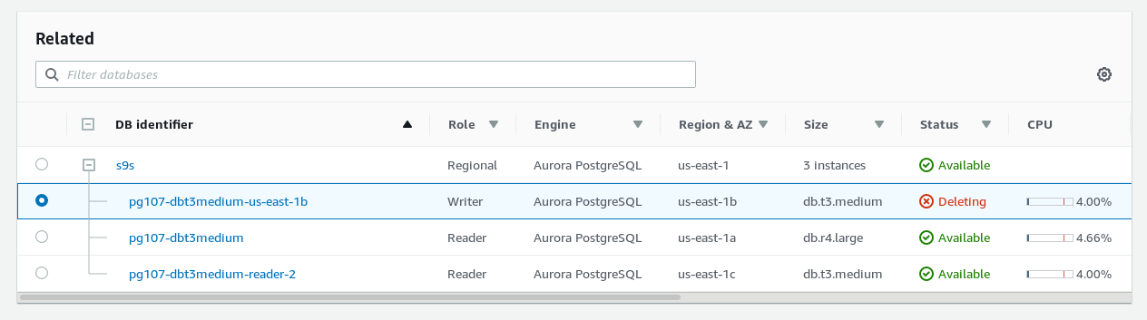
- Horizontal scaling of the primary DB instance (instance class) is not fully automatic. Before scaling the cluster triggers an automatic failover to one of the replicas. After scaling completes the new instance must be manually promoted from reader to writer:
![New instance left in reader mode after DB instance class change.]() New instance left in reader mode after DB instance class change.
New instance left in reader mode after DB instance class change.

Monitoring
- Publishing PostgreSQL logs to CloudWatch requires a minimum database engine version of 9.6.6 and 10.4.
- Only some Aurora metrics are available in the RDS Console and other metrics have different names and measurement units.
- By default, Enhanced Monitoring logs are kept in CloudWatch for 30 days.
- Cloudwatch and Enhanced Monitoring metrics will differ, as they gather data from the hypervisor and respectively the agent running on the instance.
- Performance Insights_ aggregates the metrics across all databases within a DB Instance.
- SQL statements are limited to 500 characters when viewed with AWS Performance Insights CLI and API.
Migration
- Only RDS unencrypted DB Snapshots can be encrypted at rest.
- Migrations using the Aurora Read Replica technique take several hours per TiB.
Sizing
- The smallest available instance class is db.t3.medium and the largest db.r5.24xlarge. For comparison, the MySQL engine offers db.t2.small and db.t2.medium, however no db.r5.24xlarge in the upper range.
- max_connections upper limit is 262,143.
Query Plan Management
- Statements inside PL/pgSQL functions are unsupported.
Migration
Aurora PostgreSQL does not provide direct migration services, rather the task is offloaded to a specialized AWS product, namely AWS DMS.
Conclusion
As a fully-managed drop-in replacement for the upstream PostgreSQL, Amazon Aurora PostgreSQL takes advantage of the technologies that power the AWS cloud to remove the complexity required to setup services such as auto-scaling, query load-balancing, low-level data replication, incremental backups, and encryption.
The architecture and a conservative approach for upgrading the PostgreSQL engine provides the performance and the stability organizations from small to large are looking for.
The inherent limitations are just a proof that building a large scale Database as a Service is a complex task, leaving the highly specialized PostgreSQL Hosting Providers with a niche market they can tap into.
↧
Avinash Kumar: Using plpgsql_check to Find Compilation Errors and Profile Functions

 There is always a need for profiling tools in databases for admins or developers. While it is easy to understand the point where an SQL is spending more time using
 EXPLAIN
or EXPLAIN ANALYZE
in PostgreSQL, the same would not work for functions. Recently, Jobin has published a blog post where he demonstrated how plprofiler can be useful in profiling functions.
plprofilerbuilds call graphs and creates flame graphs which make the report very easy to understand. Similarly, there is another interesting project called
plpgsql_checkwhich can be used for a similar purpose as
plprofiler, while it also looks at code and points out compilation errors. Let us see all of that in action, in this blog post.
Installing plpgsql-check
You could use yum on RedHat/CentOS to install this extension from PGDG repository. Steps to perform source installation on Ubuntu/Debian are also mentioned in the following logs.
On RedHat/CentOS
$ sudo yum install plpgsql_check_11
On Ubuntu/Debian
$ sudo apt-get install postgresql-server-dev-11 libicu-dev gcc make
$ git clone https://github.com/okbob/plpgsql_check.git
$ cd plpgsql_check/
$ make && make install
Creating and enabling this extension
There are 3 advantages of using
plpgsql_check
- Checking for compilation errors in a function code
- Finding dependencies in functions
- Profiling functions
When using plpgsql_check for the first 2 requirements, you may not need to add any entry to
shared_preload_libraries. However, if you need to use it for profiling functions (3), then you should add appropriate entries to
shared_preload_librariesso that it could load both
plpgsqland
plpgsql_check. Due to dependencies,
plpgsqlmust be before
plpgsql_checkin the
shared_preload_librariesconfig as you see in the following example :
shared_preload_libraries = plpgsql, plpgsql_check
Any change to
shared_preload_librariesrequires a restart. You may see the following error when you do not have
plpgsqlbefore
plpgsql_checkin the
shared_preload_librariesconfig.
$ grep "shared_preload_libraries" $PGDATA/postgresql.auto.conf
shared_preload_libraries = 'pg_qualstats, pg_stat_statements, plpgsql_check'

$ pg_ctl -D /var/lib/pgsql/11/data restart -mf
waiting for server to shut down.... done
server stopped
waiting for server to start....2019-07-07 02:07:10.104 EDT [6423]
FATAL: could not load library "/usr/pgsql-11/lib/plpgsql_check.so": /usr/pgsql-11/lib/plpgsql_check.so: undefined symbol: plpgsql_parser_setup
2019-07-07 02:07:10.104 EDT [6423] LOG: database system is shut down
stopped waiting
pg_ctl: could not start server
Examine the log output.

$ grep "shared_preload_libraries" $PGDATA/postgresql.auto.conf
shared_preload_libraries = 'pg_qualstats, pg_stat_statements, plpgsql, plpgsql_check'

$ pg_ctl -D /var/lib/pgsql/11/data start
.....
server started
Once the PostgreSQL instance is started, create this extension in the database where you need to perform any of the previously discussed 3 tasks.
$ psql -d percona -c "CREATE EXTENSION plpgsql_check"
CREATE EXTENSION
Finding Compilation Errors
As discussed earlier, this extension can help developers and admins determine compilation errors. But why is it needed? Let’s consider the following example where we see no errors while creating the function. By the way, I have taken this example from my previous blog post where I was talking about Automatic Index recommendations using
hypopgand
pg_qualstats. You might want to read that blog post to understand the logic of the following function.
percona=# CREATE OR REPLACE FUNCTION find_usable_indexes()
percona-# RETURNS VOID AS
percona-# $$
percona$# DECLARE
percona$#     l_queries     record;
percona$#     l_querytext     text;
percona$#     l_idx_def       text;
percona$#     l_bef_exp       text;
percona$#     l_after_exp     text;
percona$#     hypo_idx      record;
percona$#     l_attr        record;
percona$#     /* l_err       int; */
percona$# BEGIN
percona$#     CREATE TABLE IF NOT EXISTS public.idx_recommendations (queryid bigint,
percona$#     query text, current_plan jsonb, recmnded_index text, hypo_plan jsonb);
percona$#     FOR l_queries IN
percona$#     SELECT t.relid, t.relname, t.queryid, t.attnames, t.attnums,
percona$#     pg_qualstats_example_query(t.queryid) as query
percona$#       FROM
percona$#         (
percona$#          SELECT qs.relid::regclass AS relname, qs.relid AS relid, qs.queryid,
percona$#          string_agg(DISTINCT attnames.attnames,',') AS attnames, qs.attnums
percona$#          FROM pg_qualstats_all qs
percona$#          JOIN pg_qualstats q ON q.queryid = qs.queryid
percona$#          JOIN pg_stat_statements ps ON q.queryid = ps.queryid
percona$#          JOIN pg_amop amop ON amop.amopopr = qs.opno
percona$#          JOIN pg_am ON amop.amopmethod = pg_am.oid,
percona$#          LATERAL
percona$#               (
percona$#                SELECT pg_attribute.attname AS attnames
percona$#                FROM pg_attribute
percona$#                JOIN unnest(qs.attnums) a(a) ON a.a = pg_attribute.attnum
percona$#                AND pg_attribute.attrelid = qs.relid
percona$#                ORDER BY pg_attribute.attnum) attnames,
percona$#          LATERAL unnest(qs.attnums) attnum(attnum)
percona$#                WHERE NOT
percona$#                (
percona$#                 EXISTS
percona$#                       (
percona$#                        SELECT 1
percona$#                        FROM pg_index i
percona$#                        WHERE i.indrelid = qs.relid AND
percona$#                        (arraycontains((i.indkey::integer[])[0:array_length(qs.attnums, 1) - 1],
percona$#                         qs.attnums::integer[]) OR arraycontains(qs.attnums::integer[],
percona$#                         (i.indkey::integer[])[0:array_length(i.indkey, 1) + 1]) AND i.indisunique)))
percona$#                        GROUP BY qs.relid, qs.queryid, qs.qualnodeid, qs.attnums) t
percona$#                        GROUP BY t.relid, t.relname, t.queryid, t.attnames, t.attnums
percona$#     LOOP
percona$#         /* RAISE NOTICE '% : is queryid',l_queries.queryid; */
percona$#         execute 'explain (FORMAT JSON) '||l_queries.query INTO l_bef_exp;
percona$#         execute 'select hypopg_reset()';
percona$#         execute 'SELECT indexrelid,indexname FROM hypopg_create_index(''CREATE INDEX on '||l_queries.relname||'('||l_queries.attnames||')'')' INTO hypo_idx;
percona$#         execute 'explain (FORMAT JSON) '||l_queries.query INTO l_after_exp;
percona$#         execute 'select hypopg_get_indexdef('||hypo_idx.indexrelid||')' INTO l_idx_def;
percona$#         INSERT INTO public.idx_recommendations (queryid,query,current_plan,recmnded_index,hypo_plan)
percona$#         VALUES (l_queries.queryid,l_querytext,l_bef_exp::jsonb,l_idx_def,l_after_exp::jsonb);
percona$#     END LOOP;
percona$#         execute 'select hypopg_reset()';
percona$# END;
percona$# $$ LANGUAGE plpgsql;
CREATE FUNCTION
From the above log, it has created the function with no errors. Unless we call the above function, we do not know if it has any compilation errors. Surprisingly, with this extension, we can use the
plpgsql_check_function_tb()function to learn whether there are any errors, without actually calling it.
percona=# SELECT functionid, lineno, statement, sqlstate, message, detail, hint, level, position,
left (query,60),context FROM plpgsql_check_function_tb('find_usable_indexes()');
-[ RECORD 1 ]------------------------------------------------------------
functionid | find_usable_indexes
lineno     | 14
statement  | FOR over SELECT rows
sqlstate   | 42P01
message    | relation "pg_qualstats_all" does not exist
detail     |
hint       |
level      | error
position   | 306
left       | SELECT t.relid, t.relname, t.queryid, t.attnames, t.attnums,
context    |
From the above log, it is clear that there is an error where a relation used in the function does not exist. But, if we are using dynamic SQLs that are assembled in runtime, false positives are possible, as you can see in the following example. So, you may avoid the functions using dynamic SQL’s or comment the code containing those SQLs before checking for other compilation errors.
percona=# select * from plpgsql_check_function_tb('find_usable_indexes()');
-[ RECORD 1 ]------------------------------------------------------------------------------
functionid | find_usable_indexes
lineno     | 50
statement  | EXECUTE
sqlstate   | 00000
message    | cannot determinate a result of dynamic SQL
detail     | There is a risk of related false alarms.
hint       | Don't use dynamic SQL and record type together, when you would check function.
level      | warning
position   |
query      |
context    |
-[ RECORD 2 ]------------------------------------------------------------------------------
functionid | find_usable_indexes
lineno     | 52
statement  | EXECUTE
sqlstate   | 55000
message    | record "hypo_idx" is not assigned yet
detail     | The tuple structure of a not-yet-assigned record is indeterminate.
hint       |
level      | error
position   |
query      |
context    | SQL statement "SELECT 'select hypopg_get_indexdef('||hypo_idx.indexrelid||')'"
Finding Dependencies
This extension can be used to find dependent objects in a function. This way, it becomes easy for administrators to understand the objects being used in a function without spending a huge amount of time reading the code. The trick is to simply pass your function as a parameter to
plpgsql_show_dependency_tb()as you see in the following example.
percona=# select * from plpgsql_show_dependency_tb('find_usable_indexes()');
   type   |  oid  |   schema   |            name            |  params
----------+-------+------------+----------------------------+-----------
 FUNCTION | 16547 | public     | pg_qualstats               | ()
 FUNCTION | 16545 | public     | pg_qualstats_example_query | (bigint)
 FUNCTION | 16588 | public     | pg_stat_statements         | (boolean)
 RELATION |  2601 | pg_catalog | pg_am                      |
 RELATION |  2602 | pg_catalog | pg_amop                    |
 RELATION |  1249 | pg_catalog | pg_attribute               |
 RELATION |  1262 | pg_catalog | pg_database                |
 RELATION |  2610 | pg_catalog | pg_index                   |
 RELATION | 16480 | public     | idx_recommendations        |
 RELATION | 16549 | public     | pg_qualstats               |
 RELATION | 16559 | public     | pg_qualstats_all           |
 RELATION | 16589 | public     | pg_stat_statements         |
(12 rows)
Profiling Functions
This is one of the very interesting features. Once you have added the appropriate entries to
shared_preload_librariesas discussed earlier, you could easily enable or disable profiling through a GUC:
plpgsql_check.profiler.This parameter can either be set globally or for only your session. Here’s an example to understand it better.
percona=# ALTER SYSTEM SET plpgsql_check.profiler TO 'ON';
ALTER SYSTEM
percona=# select pg_reload_conf();
 pg_reload_conf
----------------
 t
(1 row)
When you set it globally, all the functions running in the database are automatically profiled and stored. This may be fine in a development or a testing environment, but you could also enable profiling of functions called in a single session through a session-level setting as you see in the following example.
percona=# BEGIN;
BEGIN
percona=# SET plpgsql_check.profiler TO 'ON';
SET
percona=# select salary_update(1000);
 salary_update
---------------

(1 row)

percona=# select lineno, avg_time, source from plpgsql_profiler_function_tb('salary_update(int)');
 lineno | avg_time |                                                    source
--------+----------+---------------------------------------------------------------------------------------------------------------
      1 |          |
      2 |          | DECLARE
      3 |          | l_abc record;
      4 |          | new_sal     INT;
      5 |    0.005 | BEGIN
      6 |   144.96 |   FOR l_abc IN EXECUTE 'SELECT emp_id, salary FROM employee where emp_id between 1 and 10000 and dept_id = 2'
      7 |          |   LOOP
      8 |      NaN |       new_sal := l_abc.salary + sal_raise;
      9 |      NaN |       UPDATE employee SET salary = new_sal WHERE emp_id = l_abc.emp_id;
     10 |          |   END LOOP;
     11 |          | END;
(11 rows)

--- Create an Index and check if it improves the execution time of FOR loop.

percona=# CREATE INDEX idx_1 ON employee (emp_id, dept_id);
CREATE INDEX
percona=# select salary_update(1000);
 salary_update
---------------

(1 row)

percona=# select lineno, avg_time, source from plpgsql_profiler_function_tb('salary_update(int)');
 lineno | avg_time |                                                    source
--------+----------+---------------------------------------------------------------------------------------------------------------
      1 |          |
      2 |          | DECLARE
      3 |          | l_abc record;
      4 |          | new_sal     INT;
      5 |    0.007 | BEGIN
      6 |   73.074 |   FOR l_abc IN EXECUTE 'SELECT emp_id, salary FROM employee where emp_id between 1 and 10000 and dept_id = 2'
      7 |          |   LOOP
      8 |      NaN |       new_sal := l_abc.salary + sal_raise;
      9 |      NaN |       UPDATE employee SET salary = new_sal WHERE emp_id = l_abc.emp_id;
     10 |          |   END LOOP;
     11 |          | END;
(11 rows)

percona=# END;
COMMIT
percona=# show plpgsql_check.profiler;
 plpgsql_check.profiler
------------------------
 on
(1 row)
In the above log, I have opened a new transaction block and enabled the parameter
plpgsql_check.profileronly for that block. So any function that I have executed in that transaction is profiled, which can be extracted using
plpgsql_profiler_function_tb(). Once we have identified the area where the execution time is high, the immediate action is to tune that piece of code. After creating the index, I have called the function again. It has now performed faster than earlier.
Conclusion
Special thanks to Pavel Stehule who has authored this extension and also to the contributors who have put this extension into a usable stage today. This is one of the simplest extensions that can be used to check for compilation errors and dependencies. While this can also be a handy profiling tool, a developer may find both plprofiler orplpgsql_check
helpful for profiling as well.
↧
Paul Ramsey: Simple SQL GIS
And, late on a Friday afternoon, the plaintive cry was heard!
Anyone got a KML/Shapefile of B.C. elxn boundaries that follows the water (Elections BC's KML has ridings going out into the sea)
— Chad Skelton (@chadskelton) November 16, 2012
And indeed, into the sea they do go!

And ‘lo, the SQL faeries were curious, and gave it a shot!
##### Commandline OSX/Linux ###### Get the Shape files# http://www.elections.bc.ca/index.php/voting/electoral-maps-profiles/
wget http://www.elections.bc.ca/docs/map/redis08/GIS/ED_Province.exe

# Exe? No prob, it's actually a self-extracting ZIP
unzip ED_Province

# Get a PostGIS database ready for the data
createdb ed_clip
psql -c"create extension postgis"-d ed_clip

# Load into PostGIS# The .prj says it is "Canada Albers Equal Area", but they# lie! It's actually BC Albers, EPSG:3005
shp2pgsql -s 3005 -i-I ED_Province ed | psql -d ed_clip

# We need some ocean! Use Natural Earth...# http://www.naturalearthdata.com/downloads/
wget http://www.naturalearthdata.com/http//www.naturalearthdata.com/download/10m/physical/ne_10m_ocean.zip
unzip ne_10m_ocean.zip

# Load the Ocean into PostGIS!
shp2pgsql -s 4326 -i-I ne_10m_ocean ocean | psql -d ed_clip

# OK, now we connect to PostGIS and start working in SQL
psql -e ed_clip
-- How big is the Ocean table?SELECTCount(*)FROMocean;-- Oh, only 1 polygon. Well, that makes it easy... -- For each electoral district, we want to difference away the ocean.-- The ocean is a one big polygon, this will take a while (if we-- were being more subtle, we'd first clip the ocean down to -- a reasonable area around BC.)CREATETABLEed_clippedASSELECTCASEWHENST_Intersects(o.geom,ST_Transform(e.geom,4326))THENST_Difference(ST_Transform(e.geom,4326),o.geom)ELSEST_Transform(e.geom,4326)ENDASgeom,e.edabbr,e.ednameFROMede,oceano;-- Check our geometry types...SELECTDISTINCTST_GeometryType(geom)FROMed_clipped;-- Oh, they are heterogeneous. Let's force them all multiUPDATEed_clippedSETgeom=ST_Multi(geom);# Dump the result out of the database back into shapes
pgsql2shp -f ed2009_ocean ed_clip ed_clipped
zip ed2009_ocean.zip ed2009_ocean.*
mv ed2009_ocean.zip ~/Dropbox/Public/
No more districts in oceans!

And the faeries were happy, and uploaded their polygons!
Update: And the lamentations ended, and the faeries also rejoiced.
@pwramsey OK, that's frickin' amazing! Thank you! Thought I was in store for hours spent editing polygons by hand in Google Earth.
— Chad Skelton (@chadskelton) November 17, 2012
↧
↧
Hubert 'depesz' Lubaczewski: Waiting for PostgreSQL 13 – Add support for –jobs in reindexdb
On 27th of July 2019, Michael Paquier committed patch: Add support for --jobs in reindexdb When doing a schema-level or a database-level operation, a list of relations to build is created which gets processed in parallel using multiple connections, based on the recent refactoring for parallel slots in src/bin/scripts/. System catalogs are processed first … Continue reading "Waiting for PostgreSQL 13 – Add support for –jobs in reindexdb"
↧
Paul Ramsey: Waiting for PostGIS 3: ST_AsMVT Performance

Vector tiles are the new hotness, allowing large amounts of dynamic data to be sent for rendering right on web clients and mobile devices, and making very beautiful and highly interactive maps possible.
Since the introduction of ST_AsMVT(), people have been generating their tiles directly in the database more and more, and as a result wanting tile generation to go faster and faster.
Every tile generation query has to carry out the following steps:
- Gather all the relevant rows for the tile
- Simplify the data appropriately to match the resolution of the tile
- Clip the data to the bounds of the tile
- Encode the data into the MVT protobuf format
For PostGIS 3.0, performance of tile generation has been vastly improved.

↧
Haroon .: PostgreSQL: Regular expressions and pattern matching
A regular expression is a special text string used to describe a search pattern. PostgreSQL’s regular expressions supports three separate approaches to pattern matching: POSIX-style regular expressions (BREs and EREs) SIMILAR TO operator added in SQL:1999 SQL LIKE operator There are some more advanced techniques for advanced pattern matching requirements but those will very likely […]
↧
Jobin Augustine: PostgreSQL: Simple C extension Development for a Novice User (and Performance Advantages)

 One of the great features of PostgreSQL is its extendability. My colleague and senior PostgreSQL developer Ibar has blogged about developing an extension with much broader capabilities including callback functionality. But in this blog post, I am trying to address a complete novice user who has never tried but wants to develop a simple function with business logic. Towards the end of the blog post, I want to show how lightweight the function is by doing simple benchmarking which is repeatable and should act as a strong justification for why end-users should do such development.
Generally, PostgreSQL and extension developers work on a PostgreSQL source build. For a novice user, that may not be required, instead, dev/devel packages provided for the Linux distro would be sufficient. Assuming that you have installed PostgreSQL already, the following steps can get you the additional development libraries required.
On Ubuntu/Debian
$ sudo apt install postgresql-server-dev-11
On RHEL/CentOS
sudo yum install postgresql11-devel
The next step is to add a PostgreSQL binary path to your environment, to ensure that pg_config is there in the path. In my Ubuntu laptop, this is how:
export PATH=/usr/lib/postgresql/11/bin:$PATH
Above mentioned paths may vary according to the environment.
Please make sure that the pg_config is executing without specifying the path:
$ pg_config
PostgreSQL installation provides a build infrastructure for extensions, called PGXS, so that simple extension modules can be built simply against an already-installed server. It automates common build rules for simple server extension modules.
$ pg_config --pgxs
/usr/lib/postgresql/11/lib/pgxs/src/makefiles/pgxs.mk
Now let’s create a directory for development. I am going to develop a simple extension addme with a function addme to add 2 numbers.
$ mkdir addme
Now we need to create a Makefile which builds the extension. Luckily, we can use all PGXS macros.
MODULES = addme
EXTENSION = addme
DATA = addme--0.0.1.sql
PG_CONFIG = pg_config
PGXS := $(shell $(PG_CONFIG) --pgxs)
include $(PGXS)
MODULE specifies the shared object without file extension and EXTENSION specifies the name of the extension name. DATA defines the installation script. The reason for –0.0.1 specifying in the name is that I should match the version we specify in the control file.
Now we need a control file addme.control with the following content:
comment = 'Simple number add function'
default_version = '0.0.1'
relocatable = true
module_pathname = '$libdir/addme'
And we can prepare our function in C which will add 2 integers:
#include "postgres.h"
#include "fmgr.h"

PG_MODULE_MAGIC;

PG_FUNCTION_INFO_V1(addme);

Datum
addme(PG_FUNCTION_ARGS)
{
int32 arg1 = PG_GETARG_INT32(0);
int32 arg2 = PG_GETARG_INT32(1);

PG_RETURN_INT32(arg1 + arg2);
}
At this stage, we have only 3 files in the directory.
$ ls
addme.c addme.control Makefile
Now we can make the file:
$ make
For installing the extension, we need a SQL file with create function. This SQL file name should be the same as the one we specified in DATA parameter in the Makefile, which is addme–0.0.1.sql
Add the following content into this file:
CREATE OR REPLACE FUNCTION
addme(int,int) RETURNS int AS 'MODULE_PATHNAME','addme'
LANGUAGE C STRICT;
And install the extension:
$ sudo make install
Now we can proceed to create the extension and test it:
postgres=# create extension addme;
CREATE EXTENSION
postgres=# select addme(2,3);
addme
-------
5
(1 row)
Just like any function, we can use it in queries against multiple tuples.
postgres=# select 7||'+'||g||'='||addme(7,g) from generate_series(1,10) as g;
?column?
----------
7+1=8
7+2=9
7+3=10
7+4=11
7+5=12
7+6=13
7+7=14
7+8=15
7+9=16
7+10=17
(10 rows)
Performance Benchmarking
Now it is important to understand the performance characteristics calling a C function in extension. For comparison, we have two options like:
1. ‘+’ operator provided by SQL like
select 1+2;
2. PLpgSQL function as below
CREATE FUNCTION addmepl(a integer, b integer)
 RETURNS integer
as $$
BEGIN
  return a+b;
END;
$$ LANGUAGE plpgsql;
For this test/benchmark, I am going to call the function for 1 million times!
SQL + operator
time psql -c "select floor(random() * (100-1+1) + 1)::int+g from generate_series(1,1000000) as g" > out.txt
C function call
$ time psql -c "select addme(floor(random() * (100-1+1) + 1)::int,g) from generate_series(1,1000000) as g" > out.txt
PL function call
$ time psql -c "select addmepl(floor(random() * (100-1+1) + 1)::int,g) from generate_series(1,1000000) as g" > out.txt
I have performed the tests 6 times for each case and tabulated below.
Test Run

As we can see, the performance of Built in ‘+’ operator and the custom C function in the extension takes the least time with almost the same performance. But the PLpgSQL function call is slow and it shows considerable overhead. Hope this justifies why those functions, which are heavily used, need to be written as a native C extension.
↧
↧
Sven Klemm: OrderedAppend: An optimization for range partitioning

With this feature, we’ve seen up to 100x performance improvements for certain queries.
In our previous post on implementing constraint exclusion, we discussed how TimescaleDB leverages PostgreSQL’s foundation and expands on its capabilities to improve performance. Continuing with the same theme, in this post we will discuss how we’ve added support for ordered appends which optimize a large range of queries, particularly those that are ordered by time.
We’ve seen performance improvements up to 100x for certain queries after applying this feature, so we encourage you to keep reading!
Optimizing Appends for large queries
PostgreSQL represents how plans should be executed using “nodes”. There are a variety of different nodes that may appear in an EXPLAIN output, but we want to focus specifically on Append nodes, which essentially combine the results from multiple sources into a single result.
PostgreSQL has two standard Appends that are commonly used that you can find in an EXPLAIN output:
- Append: appends results of child nodes to return a unioned result
- MergeAppend: merge output of child nodes by sort key; all child nodes must be sorted by that same sort key; accesses every chunk when used in TimescaleDB
When MergeAppend nodes are used with TimescaleDB, we necessarily access every chunk to figure out if the chunk has keys that we need to merge. However, this is obviously less efficient since it requires us to touch every chunk.
To address this issue, with the release of TimescaleDB 1.2 we introduced OrderedAppend asan optimization for range partitioning. The purpose of this feature is to optimize a large range of queries, particularly those that are ordered by time and contain a LIMIT clause. This optimization takes advantage of the fact that we know the range of time held in each chunk, and can stop accessing chunks once we’ve found enough rows to satisfy the LIMIT clause. As mentioned above, with this optimization we see performance improvements of up to 100x depending on the query.
With the release of TimescaleDB 1.4, we wanted to extend the cases in which OrderedAppend can be used. This meant making OrderedAppend space-partition aware, as well as removing the LIMIT clause restriction from Ordered Append. With these additions, more users can benefit from the performance benefits achieved through leveraging OrderedAppend.
(Additionally, the updates to OrderedAppend for space partitions will be leveraged even more heavily with the release of TimescaleDB clustering which is currently in private beta. Stay tuned for more information!)
Developing query plans with the optimization
As an optimization for range partitioning, OrderedAppend eliminates sort steps because it is aware of the way data is partitioned.
Since each chunk has a known time range it covers to get sorted output, no global sort step is needed. Only local sort steps have to be completed and then appended in the correct order. If index scans are utilized, which return the output sorted, sorting can be completely avoided.
For a query ordering by the time dimension with a LIMIT clause you would normally get something like this:
dev=# EXPLAIN (ANALYZE,COSTS OFF,BUFFERS,TIMING OFF,SUMMARY OFF)
dev-# SELECT * FROM metrics ORDER BY time LIMIT 1;
                                                 QUERY PLAN
------------------------------------------------------------------------------------------------------------
 Limit (actual rows=1 loops=1)
   Buffers: shared hit=16
   ->  Merge Append (actual rows=1 loops=1)
         Sort Key: metrics."time"
         Buffers: shared hit=16
         ->  Index Scan using metrics_time_idx on metrics (actual rows=0 loops=1)
               Buffers: shared hit=1
         ->  Index Scan using _hyper_1_1_chunk_metrics_time_idx on _hyper_1_1_chunk (actual rows=1 loops=1)
               Buffers: shared hit=3
         ->  Index Scan using _hyper_1_2_chunk_metrics_time_idx on _hyper_1_2_chunk (actual rows=1 loops=1)
               Buffers: shared hit=3
         ->  Index Scan using _hyper_1_3_chunk_metrics_time_idx on _hyper_1_3_chunk (actual rows=1 loops=1)
               Buffers: shared hit=3
         ->  Index Scan using _hyper_1_4_chunk_metrics_time_idx on _hyper_1_4_chunk (actual rows=1 loops=1)
               Buffers: shared hit=3
         ->  Index Scan using _hyper_1_5_chunk_metrics_time_idx on _hyper_1_5_chunk (actual rows=1 loops=1)
               Buffers: shared hit=3
You can see 3 pages are read from every chunk and an additional page from the parent table which contains no actual rows.
While with this optimization enabled you would get a plan looking like this:
dev=# EXPLAIN (ANALYZE,COSTS OFF,BUFFERS,TIMING OFF,SUMMARY OFF)
dev-# SELECT * FROM metrics ORDER BY time LIMIT 1;
                                                 QUERY PLAN
------------------------------------------------------------------------------------------------------------
 Limit (actual rows=1 loops=1)
   Buffers: shared hit=3
   ->  Custom Scan (ChunkAppend) on metrics (actual rows=1 loops=1)
         Order: metrics."time"
         Buffers: shared hit=3
         ->  Index Scan using _hyper_1_1_chunk_metrics_time_idx on _hyper_1_1_chunk (actual rows=1 loops=1)
               Buffers: shared hit=3
         ->  Index Scan using _hyper_1_2_chunk_metrics_time_idx on _hyper_1_2_chunk (never executed)
         ->  Index Scan using _hyper_1_3_chunk_metrics_time_idx on _hyper_1_3_chunk (never executed)
         ->  Index Scan using _hyper_1_4_chunk_metrics_time_idx on _hyper_1_4_chunk (never executed)
         ->  Index Scan using _hyper_1_5_chunk_metrics_time_idx on _hyper_1_5_chunk (never executed)
After the first chunk, the remaining chunks never get executed and to complete the query only 3 pages have to be read. TimescaleDB removes parent tables from plans like this because we know the parent table does not contain any data.
MergeAppend vs. ChunkAppend
The main difference between these two examples is the type of Append node we used. In the first case, a MergeAppend node is used. In the second case, we used a ChunkAppend node (also introduced in 1.4) which is a TimescaleDB custom node that works similarly to the PostgreSQL Append node, but contains additional optimizations.
The MergeAppend node implements the global sort and requires locally sorted input which has to be sorted by the same sort key. To produce one tuple, the MergeAppend node has to read one tuple from every chunk to decide which one to return to.
For the very simple example query above, you will see 16 pages read (with MergeAppend) vs. 3 pages (with ChunkAppend) which is a 5x improvement over the unoptimized case (if we ignore the single page from the parent table), and represents the number of chunks present in that hypertable. So for a hypertable with 100 chunks, there would be 100 times less pages to be read to produce the result for the query.
As you can see, you gain the most benefit from OrderedAppend with a LIMIT clause as older chunks don’t have to be touched if the required results can be satisfied from more recent chunks. This type of query is very common in time-series workloads (e.g. if you want to get the last reading from a sensor). However, even for queries without a LIMIT clause, this feature is beneficial because it eliminates sorting of data.
Next steps
If you are interested in using OrderedAppend, make sure you have TimescaleDB 1.2 or higher installed (installation guide). However, we always recommend upgrading to the most recent version of the software (at the time of publishing this post, it’s TimescaleDB 1.4).
If you are brand new to TimescaleDB, get started here. Have questions? Join our Slack channel or leave them in the comments section below.
↧
Konstantin Evteev: Standby in production: scaling application in second largest classified site in the world.
Standby in production: scaling application in the second largest classified site in the world

Hi. My name is Konstantin Evteev, I’m a DBA Unit Leader of Avito. Avito is the biggest Russian classified site, and the second largest classified site in the world (after Craigslist of USA). Items offered for sale on Avito can be brand new or used. The website also publishes job vacancies and CVs.
Via its web and mobile apps, the platform monthly serves more than 35 million users. They add approximately a million new ads a day and close over 100,000 transactions per day. The back office has accumulated more than a billion ads. According to Yandex, in some Russian cities (for example, in Moscow), Avito is considered a high load project in terms of page views. Some figures can give a better idea of the project’s scale:
- 600+ servers;
- 4.5 Gbit/sec TX, 2 Gbit/sec RX without static;
- about a million queries per minute to the backend;
- 270TB of images;
- >20 TB in Postgres on 100 nodes:
- 7–8K TPS on most nodes;
- the largest — 20k TPS, 5 TB.
At the same time, these volumes of data need not only to be accumulated and stored but also processed, filtered, classified and made searchable. Therefore, expertise in data processing is critical for our business processes.
The picture below shows the dynamic of pageviews growth.
Our decision to store ads in PostgreSQL helps us to meet the following scaling challenges: the growth of data volume and growth of number of requests to it, the scaling and distribution of the load, the delivery of data to the DWH and the search subsystems, inter-base and internetwork data synchronization, etc. PostgreSQL is the core component of our architecture. Reach set of features, legendary durability, built-in replication, archive, reserve tools are found a use in our infrastructure. And professional community helps us to effectively use all these features.
In this report, I would like to share Avito’s experience in different cases of standby usage in the following order:
- a few words about standby and its history in general;
- problems and solutions in replication based horizontal scale-out;
- Avito’s implementation for solution to avoid stale reads from replica;
- possible pitfalls while using standby with high request rate, applying DDL, receiving WAL files from the archive;
- handling issues with technique of using several standbys in production and routing queries between them;
- logical replication based scaling example to compare;
- conclusions and standby major upgrade features.
A few words about standby and its history in general
Standby can be used for the following purposes.
- High availability: if primary crashes you need to have hot reserve to make fast failover
- Scaling — you can switch part or all your read queries between one or more standbys
In early 2000s, PostgreSQL community didn’t think that replication should be a built-in feature. Vadim Mikheev after implementation of MVCC, developed a replication solution «Rserv» based on MVCC internal mechanics. The following logic was supposed to be used to replicate data: taking changes that were not visible in a previous snapshot and became visible in the current snapshot. Then Jan Wieck developed an enterprise logical replication solution based on Vadim Mikheev’s idea and named it Slony (Russian for “elephant”) as a reverence for its author. Then the team from Skype created SkyTools with PgQ (the transactional queue) and Londiste (the logical replication solution based on PgQ). PostgreSQL 8.3 аdd several txid_*() functions to query active transaction IDs. This is useful for various replication solutions. (Jan). And finally Logical replication became a built-in feature in PostgreSQL 10.
Meanwhile, built-in binary replication was evolving.
- 2001 PostgreSQL 7.1: write-ahead log is created to improve write performance.
- 2005 PostgreSQL 8.0: point in time recovery, makes it possible to create handmade replication scripts to have warm reserve.
- 2008 PostgreSQL 8.3: administration of previously released warm standby feature (2006) becomes easier. That’s why someone still uses PostgreSQL 8.3 in production.
- 2010 PostgreSQL 9.0: since this version PostgreSQL standby has been able to serve read queries (hot standby), moreover release of streaming replication feature has simplified setting up replication and decreased possible replication lag.
- 2011 PostgreSQL 9.1: synchronous replication makes it easier to support SLA for applications working with critical data (for example information about financial transactions). Previously to avoid data loss you had to wait until your data was successfully replicated to standby or had to save data in two databases manually.
- 2013 PostgreSQL 9.3: standby can follow timeline switch which makes failover procedures easier.
- 2014 PostgreSQL 9.4: replication slots make it safer to setup standby without archive, but as a result standby fail can lead to master fail. Logical decoding becomes the fundament for built-in logical replication.
- 2016 PostgreSQL 9.6: multiple synchronous standbys give an opportunity to create more reliable clusters. Remote_apply makes it possible to serve read queries from standby without stale reads.
So we have discussed few classifications of standby: logical and physical, built-in and stand alone solutions, read only and not only read only, sync and async.
Now let’s look closer at physical built-in read only async standbу.
In Streaming Replication, three kinds of processes work together. A walsender process on the primary server sends WAL data to а standby server; and then, a walreceiver and startup processes on standby server receives and replays these data. A walsender and a walreceiver communicate using a single TCP connection.
Problems and solutions in replication based horizontal scale-out
When you use asynchronous standby, it can fall behind the primary. That’s why different rules for routing read queries to the primary or to the standby match different types of applications.
- First approach — don’t use any routing technique, just route any read query to standby. For some applications it will be good due to many reasons such as:
- low replication lag;
- specific profile of queries with a lack of or a small number of errors connected with stale reads;
- and so on.
But I don’t like this approach, let’s look at better techniques for routing read queries to standby.
2. Sometimes there is a specific business logic that can allow exploiting stale reads. For example, few years ago on Avito there was a 30-minute interval before our users could see new ads (time for anti-fraud check and other restrictions). So we successfully use this specific business rule for routing your read queries for other people’s ads. At the same time we route read queries to your own ads to the primary. Thus, you may edit your own ad and work with the actual ad’s state. To make this routing approach work in a correct way we need to support a replication lag lower than the 30-minute interval.
3. There can be situations when stale reads are not acceptable, even more interesting when you need to use few standbys to achieve a greater level of scale. To deal with them you need to use special techniques. Let’s look closer at our example and the technique to avoid stale reads
Avito’s implementation to avoid stale reads from replica
We successfully used the logical routing technique (number 2: based on business specific logic) when we faced the following spikes. In the picture you can see a diagram with the Load Average on a 28-physical-core machine (2X Intel(R) Xeon(R) CPU E5–2697 v3 @ 2.60GHz). When we started using Hyper-threading, we benchmarked and found out that most of our queries were successfully scaled with enabling Hyper-threading. But then the distribution of queries changed and the result of this can be seen on the diagram. When the level of load average got closer to the number of physical cores, the spikes happened.
The same spikes were observed on the CPU diagram below. From my side, I saw that all queries started being executed dozens of times longer.
So I experienced the capacity problem of the primary server. Actually, the capacity of one server is bounded by the most powerful market offering. If it does not fit you, it is a capacity problem. Normally, changing the architecture of your application is not so that fast and moreover it might be complicated and take a lot of time. Being under such circumstances I had to find a quick solution. As you can notice that the spikes are gone, we coped with the capacity problem by switching more read queries to standby (you can see the number of queries on standby on the following TPS diagram).
We distributed load among more nodes in the system by re-routing queries that don’t need to run on the primary. The main challenges in spreading read queries to replicas are stale reads and race conditions.
On the links you can see detailed description of routing reads based on replica WAL position technique. The main idea is to store the last committed LSN for the entity on which mutating request was executed. Then, when we subsequently want to fulfill a read operation for the same entity, we’ll check which replicas have consumed to that point or beyond it, and randomly select one from the pool. If no replicas are sufficiently advanced (i.e. say a read operation is being run very closely after the initial write), we’ll fall back to the master. Stale reads become impossible regardless of the state of any given replica.
We made some simplification in the technique above. We didn’t use exactly the same one because we didn’t have enough time and resources to rewrite application by implementing sticky connections based on LSN tracking.
At that time we were facing the capacity problem of the primary server, we had a huge monolithic application (it was in progress of splitting to microservice architecture). So it had a lot of complicated logic and deep nested calls — which forced us to make migration to sticky LSN sessions unreachable in short term period. But on the other hand, we had some historical background: we had a timestamp column in the user and the item tables (our main entities), which we filled with the help of PostgreSQL function now(): current date and time — start of current transaction. So we decided to use timestamp instead of LSN. Probably you know that timestamp can’t be used for the task of serialization data operations (or tracking position of replica in relation to primary) in PostgreSQL. To make this assumption we used the following arguments:
- we didn’t have long transactions (all of them lasted several milliseconds);
- we routed all read queries for the entity on which mutating request was executed within 7.5 minutes to primary server;
- we could route read queries to replicas, which must not fall behind in relation to primary greater than 5-minute interval.
Eventually, we came up with the following solution (we called it Avito Smart Cache). We replaced our cache based on Redis with the one implemented in Tarantool. (Tarantool is a powerful fast data platform that comes with an in-memory database and an integrated application server).
We made two levels of cache. The first level — the hot cache — stores sticky sessions. Sticky connections are supported by storing the timestamp of last user’s data mutation. Each user is given its own key so that the actions of one user would not lead to all other users being affected.
Let’s look closer at the approach we used to deliver user’s timestamp information to Tarantool. We have made some changes in our framework for working with database: we have added «on commit hook». In this «hook» we invoke sending data mutation’s timestamp to the 1st level of cache. You may notice, that there is a possibility when we successfully have made changes in PostgreSQL database but couldn’t deliver this info to cache (for example there was a network problem or application error or smth else). To deal with such cases we have made the Listener. All mutations on the database side are sent to the Listener using PostgreSQL LISTEN and NOTIFY features. Also, the Listener tracks last_xact_replay_timestamp of standby and has HTTP API from which Tarantool takes this information.
The second level is the cache for our read data to minimize utilization of PostgreSQL resources (replacing the old cache in Redis).
Some special features:
- On the schema there are 16 Tarantool shards to help us to be resilient. When 1 shard crashes, PostgreSQL can continue processing 1/16 queries without help of the cache.
- Decreasing the value of time interval used for routing queries causes the growth in number of queries to standby. Meanwhile, this leads to increasing probability that standbys lag is greater than the routing interval. If this happens, all queries will be sent to the primary server and it’s highly likely that the primary won’t be able to process all these requests. And this elicits one more fact: when you use 2 nodes (primary and standby in production), you need at least the 3rd node (2nd standby) for the reserve purpose, and there should be a disaster recovery plan for all parts of this complex infrastructure.
The main logic of working with smart cache is as follows.
Trying to find data on the main level of the cache, if we find it, it is success. If we do not then we try to get data on the 1st level hot cache. If we find data in the hot cache, it means that there were recent changes in our data and we should get data from primary.
Or if the standbys lag is greater than routing interval — we also should get data from the primary.
Otherwise, data hasn’t been changed for a long time and we can route read request to standby.
You may notice different ttl values — they are different because there is a probability of races and In cases where the probability is greater I use smaller ttl to minimize losses.
Thus we successfully implemented one of the techniques for routing queries and made eventually synchronized cache. But on the graph below you may notice the spikes. These spikes appeared when standby started falling behind due to some reasons such as different locks or specific profile of utilizing hardware resources. In the following part of my report, I would like to share Avito’s experience in solving those issues on the standbys.
Сases highlighting possible problems while using standby with high request rate, applying DDL, receiving WAL files from archive and handling some issues with technique of using few standbys in production and routing queries between them
1st: Deadlock on standby
Step 1:
The Infrastructure for this case is as follows:
- primary (master);
- standby;
- two tables: the items and the options.
Step 2
Open transaction on the primary and alter the options table.
Step 3
On the standby execute the query to get data from the items table.
Step 4
On the primary side alter the items table.
Step 5
Execute the query to get data from the items table.
In PostgreSQL versions lower than 10 we have a deadlock that is not detected. Such deadlocks have successfully been detected by deadlock detector since PostgreSQL 10.
2nd: DDL (statement_timeout and deadlock_timeout)
The infrastructure for this case is the same.
How to apply DDL changes to the table, receiving thousands read requests per second. Of course with the help of statement_timeout setting (Abort any statement that takes more than the specified number of milliseconds, starting from the time the command arrives at the server from the client. ).
Another setting you should use to apply DDL is deadlock_timeout. This is the amount of time, in milliseconds, to wait on a lock before checking to see if there is a deadlock condition. The check for deadlock is relatively expensive, so the server doesn’t run it every time it waits for a lock. We optimistically assume that deadlocks are not common in production applications and just wait on the lock for a while before checking for a deadlock. Increasing this value reduces the amount of time wasted in needless deadlock checks, but slows down reporting of real deadlock errors. The default is one second (1s), which is probably about the smallest value you would want in practice. On a heavily loaded server you might want to raise it. Ideally the setting should exceed your typical transaction time, so as to improve the odds that a lock will be released before the waiter decides to check for deadlock.
Deadlock timeout setting controls the time when conflicting autovacuum is canceled, because the default 1-second value is also the value of duration of the lock while applying DDL and it can lead to a trouble in systems with thousands requests per second.
There is some specifics in the scope of statement_timeout setting and the changes take effect ( for example changing statement_timeout inside the stored procedure will take no effect on this procedure call).
With the help of the settings above we repeatedly try to apply changes to the structure of our tables with a short lock (approximately dozens of ms). Sometimes we can’t do this (take a lock within dozens of ms) during the daytime, and then we try to do it at night, when the traffic rate is lower. Usually we manage to do it. Otherwise we increase the values of those settings(«time window» for getting the lock).
After execution of the DDL statement with timeouts on the primary, these changes are replicated to standby. Timeouts aren’t replicated to the standby that’s why there may be locks between the WAL replay process and read queries.
2018–01–12 16:54:40.208 MSK pid=20949,user=user_3,db=test,host=127.0.0.1:55763 LOG: process 20949 still waiting for AccessShareLock on relation 10000 of database 9000 after 5000.055 ms
2018–01–12 16:54:40.208 MSK pid=20949,user=user_3,db=test,host=127.0.0.1:55763 DETAIL: Process holding the lock: 46091. Wait queue: 18639, 20949, 53445, 20770, 10799, 47217, 37659, 6727, 37662, 25742, 20771,
We have implemented the workaround to deal with the issue above. We use the proxy to route queries to one of two standbys. And when we want to apply the DDL command on the primary, we stop replaying of the replication on the standby where the queries are executed.
- Wait till the ALTER command is replayed on the second standby.
- Then switch traffic to the second standby (which has successfully replayed the WAL with DDL statement).
- Start the replication on the first standby and wait till the ALTER command has been replayed on it.
Return the first standby to the pool of active standbys.
3rd: Vacuum replaying on standby and truncating data file
Vacuum can truncate the end of data file — the exclusive lock is needed for this action. At this moment on the standby long locks between read only queries and recovery process may occur. It happens because some unlock actions are not written to WAL. The example below shows a few AccessExclusive locks in one xid 920764961, and not a single unlock… Unlock happens much later. When the standby replays the commit.
The solution for that issue can be like:
- skip table truncation at VACUUM is coming in PostgreSQL 12;
- decrease the number of locks on standby (Postgres Professional idea).
In our case (when we faced problem above) we have a kind of table with logs. Almost append only — once a week we executed a delete query with timestamp condition, we cleaned records older than 2 weeks. This specific workload makes it possible to truncate the end of the data files with the autovacuum process. At the same time we actively use the standby for reading queries. The consequences can be seen above. Eventually we successfully solved that issue by executing cleaning queries more frequently: every hour.
4th: Restoring WAL from archive
On Avito we actively use standbys with the replication being set up with the help of an archive. This choice was made to have an opportunity to recreate any crashed node ( primary or standby) from the archive and then set it in a consistent state in relation to the current primary.
In 2015, we faced the following situation: some of our services started generating too many WAL files. As a result our archive command reached up the performance limits, you may notice the spikes with pending WAL files for sending to the archive on the graph below.
You can notice the green arrow pointing to the area, where we solved this issue. We implemented multithreaded archive command.
You can make a deep dive into the implementation following the github link. In short, it has the following logic: if the number of ready WAL files is lower than the threshold value, then the archive is to be done with one thread, else turn on a parallel archive technique.
But then we were faced the problem of CPU utilization on the standby. It was not obvious at first view that we were monitoring CPU utilization for our profile of load in a wrong way. Getting /proc/stat values we can see just a snapshot of the current CPU utilization. Archiving one WAL file in our case takes 60 ms and on the snapshots we don’t see the whole picture. The details could be seen with the help of the counter measurements.
Due to the above reasons there was a challenge for us to find the true answer why the standby was falling behind in relation to the primary (almost all standby CPU resources were utilized by archiving and unarchiving WAL files). The green arrow on the schema above shows the result of the optimization in the standby CPU usage. This optimization was made in a new archive schema, by delegating the archiving command execution to the archive server.
First let’s look under the hood of the old archive schema. The archive is mounted to the standby with the help of NFS. The primary sends the WAL files to archive through the standby (on this standby users’ read queries are routed to minimize the replication lag). The archive command includes the compression step, and it is carried out by the CPU of the standby server.
New archive schema:
- Compression step is carried out by the archive server CPU.
- Archive is not the single point of failure. WAL is normally archived in two archives, or at least in one (in case another one is crashed or becomes unavailable). Running synchronizing WAL files procedure after each backup is the way to deal with temporary unavailability of one of two archives servers.
- With the help of new archive schema we expanded the interval for PITR and the number of backups. We use the archives in turn, for example, 1st backup on 1st archive, 2nd backup on 2nd archive, 3rd backup on 1st archive, 4th backup on 2nd archive.
Both archive solutions were ideas of Michael Tyurin further developed by Sergey Burladyan and implemented by Victor Yagofarov. You can get it here. The solutions above were made for PostgreSQL versions where pg_rewind and pg_receivexlog were not available. With its help it is easier to deal with crashes in the distributed PostgreSQL infrastructure based on asynchronous replication. You can see the example of a crash of the primary at the schema below and there can be variants:
- some changes have been transferred neither to the standby nor to the archive;
- all the data has been transferred either to the standby or to the archive. In other words, the archive and the standby are in different states.
So there can be different cases with many «IFs» in your Disaster Recovery Plan. On the other hand, when something goes wrong it is harder to concentrate and to do everything right (for example). That’s why DRP must be clear to responsible stuff and be automated. There is a really beneficial report named «WARM standby done right» by Heikki Linnakangas where you can find a good overview and description of the tooling and the techniques to make warm standby.
Besides I want to share one configuration example of PostgreSQL infrastructure from my experience. Even using synchronous replication for standby and archive, it may happen that the standby and the archive are in different states after a crash of the primary. Synchronous replication works in such a manner: on the primary changes are committed, but there is a data structure in memory(it is not written to the WAL) that indicates that clients can’t see these changes. That indicator is stored until synchronous replicas send acknowledgment that they have successfully replayed the changes above.
Standbys pool
The existence of the possible lag of standby and other problems I have described above made us use the standbys pool in Avito’s infrastructure.
With the help of HAProxy and check function, we altered few standbys. The idea is that when the standby lag value is greater than the upper border, we close it for users’ queries until the lag value is smaller than the lower border.
if master
then false
if lag > max
then create file and return false
if lag > min and file exists
then return false
if lag < min and file exists
then remove file and return true
else
true
To implement this logic we need to make a record on the standby side. It can be implemented with the help of foreign data wrapper or untrusted languages(PL/Perl, PL/Python and etc).
Logical replication as an alternative tool to scale application
It is out of the current topic but I want to say that there is logical replication as an alternative of binary replication. With its help, the following Avito’s issues are successfully solved: the growth of data volume and growth of number of requests to it, the scaling and the distribution of the load, the delivery of data to the DWH and to the search subsystems, inter-base and intersystem data synchronization, etc. Michael Tyurin (ex chief architect) is the author of the majority of core solutions mentioned above, implemented with the help of SkyTools.
Both kinds of replication solutions have their strengths and weaknesses. Since PostgreSQL 10 logical replication has been a built-in feature. Andhere is an article with Avito’s recovery cases and techniques.
One of successful examples of logical replication usage in Avito is the organization of search results preview (since 2009 to the 1st quarter 2019). The idea is in making trigger-based materialized view (www.pgcon.org/2008/schedule/attachments/64_BSDCan2008-MaterializedViews-paper.pdf, www.pgcon.org/2008/schedule/attachments/63_BSDCan2008-MaterializedViews.pdf ), and then replicating it to another machine for read queries.
This Machine is much cheaper than the main server. And as a result, we serve all our search results from this node. On the graph below you can find information about TPS and CPU usage: it is very effective pattern of scale read load.
There are a lot more things to discuss such as reserve for logical replica, unlogged tables to increase performance, pros and cons and so on. But it is a completely different story and I will tell it next time. The point I want to highlight is that using logical replication can be very useful in many cases. There are no such drawbacks as in streaming replication, but it also has its own operation challenges. As a result there is no «silver bullet», knowledge about both types of replication helps us make the right choice in a specific case.
Conclusions
There are a few types of standby and each fits a specific case. When I was going to start preparing this report I intended to make the following conclusion. There are many operation challenges, that’s why it is better to scale your application with sharding. With the help of standby these tasks can be done without extra efforts:
- hot reserve;
- analytical queries;
- read queries when stale reads is not a problem.
Moreover, I was going to stop using binary standby for reading queries in Avito production. But opportunities have changed and we are going to build multi-datacenter architecture. Each service should be deployed at least in 3 datacenters. This is how the deploy schema looks like: a group of instances of each microservice and one node of its database (primary or standby) should be located in each data center. Reads will be served locally whereas writes will be routed to the primary.
So the opportunities make us use standby in production.
I have described several approaches and techniques above how to serve reads from standby. There are some pitfalls and a few of them have been found and successfully solved by us. Built-in solutions for pitfalls mentioned in this report could make standby operating experience better. For example, some kind of hints to write deadlock and statement timeout to WAL. If you are aware of other pitfalls let’s share that knowledge with us and the community.
Another crucial moment — is to make backups and reserve right way. Create your disaster recovery plan, support it in actual state with regular drills. Moreover, in order to minimize downtime period automize your recovery. One more aspect about reserve and standby is that if you use standby in production to execute application queries you should have another one for reserve purposes.
Suppose you have to do major upgrade and you can’t afford a long downtime. With primary and standby in production there is a high probability that one node can’t serve all queries (after the upgrade you should also have two nodes). To do this fast you can either use logical replication or upgrade master and standby with pg_upgrade. On Avito we use pg_upgrade. From the documentation, it is not obvious how to do it right if your standby receives WAL files from archive. If you use Log-Shipping standby servers (without streaming), the last file in which shutdown checkpoint record is written won’t be archived. To make the standby servers caught up you need to copy the last WAL file from primary to the standby servers and wait till it is applied. After that standby servers can issue restart point at the same location as in the stopped master. Alternatively, you can switchfrom Log-Shipping to Streaming Replication.
Yet another useful example from my upgrade experience.
In production config vacuum_defer_cleanup_age = 900000. With this setting pg_upgrade cannot freeze pg_catalog in a new cluster (it executes ‘vacuumdb — all — freeze’) during performing upgrade and upgrade fails:
Performing Upgrade
------------------
Analyzing all rows in the new cluster ok
Freezing all rows on the new cluster ok
Deleting files from new pg_clog ok
Copying old pg_clog to new server ok
Setting next transaction ID and epoch for new cluster ok
Deleting files from new pg_multixact/offsets ok
Copying old pg_multixact/offsets to new server ok
Deleting files from new pg_multixact/members ok
Copying old pg_multixact/members to new server ok
Setting next multixact ID and offset for new cluster ok
Resetting WAL archives ok
connection to database failed: FATAL: database "template1" does not exist
could not connect to new postmaster started with the command:
"/home/test/inst/pg9.6/bin/pg_ctl" -w -l "pg_upgrade_server.log" -D "new/"
-o "-p 50432 -b -c synchronous_commit=off -c fsync=off -c
full_page_writes=off -c listen_addresses='' -c unix_socket_permissions=0700
-c unix_socket_directories='/home/test/tmp/u'" start
Failure, exiting
Test script:
#!/bin/bash
PGOLD=~/inst/pg9.4/bin
PGNEW=~/inst/pg9.6/bin
${PGOLD}/pg_ctl init -s -D old -o "--lc-messages=C -T pg_catalog.english"${PGNEW}/pg_ctl init -s -D new -o "--lc-messages=C -T pg_catalog.english"echo vacuum_defer_cleanup_age=10000 >> new/postgresql.auto.conf
# move txid to 3 000 000 000 in old cluster as in production
${PGOLD}/pg_ctl start -w -D old -o "--port=54321--unix_socket_directories=/tmp"
${PGOLD}/vacuumdb -h /tmp -p 54321 --all --analyze${PGOLD}/vacuumdb -h /tmp -p 54321 --all --freeze${PGOLD}/pg_ctl stop -D old -m smart#
${PGOLD}/pg_resetxlog -x 3000000000 olddd if=/dev/zero of=old/pg_clog/0B2D bs=262144 count=1
# # move txid in new cluster bigger than vacuum_defer_cleanup_age may fix
problem
# ${PGNEW}/pg_ctl start -w -D new -o "--port=54321--unix_socket_directories=/tmp"
# echo "select txid_current();" | ${PGNEW}/pgbench -h /tmp -p 54321 -n -P 5-t 100000 -f- postgres
# ${PGNEW}/pg_ctl stop -D new -m smart${PGNEW}/pg_upgrade -k -d old/ -D new/ -b ${PGOLD}/ -B ${PGNEW}/# rm -r new old pg_upgrade_* analyze_new_cluster.sh delete_old_cluster.sh
I did not find any prohibition in the documentation on using production config with pg_upgrade, maybe I am wrong and this has already been mentioned in the documentation.
I and my colleagues are hoping to see improvements in replication in future PostgreSQL versions. Both replication approaches in PostgreSQL are a great achievement, it is very simple today to set up replication with high performance. This article is written to share Avito experience and highlight main demands of Russian PostgreSQL community (I suppose that members of PostgreSQL community worldwide face the same problems).
Standby in production: scaling application in second largest classified site in the world. was originally published in AvitoTech on Medium, where people are continuing the conversation by highlighting and responding to this story.
↧
Luca Ferrari: Checking PostgreSQL Version in Scripts
psql(1) has a bar support for conditionals, that can be used to check PostgreSQL version and act accordingly in scripts.
Checking PostgreSQL Version in Scripts
psql(1) provides a little support to conditionals and this can be used in scripts to check, for instance, the PostgreSQL version.
This is quite trivial, however I had to adjust an example script of mine to act properly depending on the PostgreSQL version.
The problem
The problem I had was with declarative partitioning: since PostgreSQL 11, declarative partitioning supports a DEFAULT partition, that is catch-all bucket for tuples that don’t have an explicit partition to go into. In PostgreSQL 10 you need to manually create catch-all partition(s) by explicitly defining them.
In my use case, I had a set of tables partitioned by a time range (the year, to be precise), but I don’t want to set up a partition for each year before the starting point of clean data: all data after year 2015 is correct, somewhere there could be some dirty data with bogus years.
Therefore, I needed a partition to catch all bogus data before year 2015, that is, a partition that ranges from the earth creation until 2015. In PostgreSQL 11 this, of course, requires you to define a DEFAULT partition and that’s it! But how to create a different default partition on PostgreSQL 10 and 11?
I solved the problem with something like the following:
\if:pg_version_10\echo'PostgreSQL version is 10'\echo'Emulate a DEFAULT partition'CREATETABLEdigikam.images_oldPARTITIONOFdigikam.images_rootFORVALUES ↧